This is legacy documentation covering MuJoCo versions 2.0 and earlier. Updated documentation is available from DeepMind at www.mujoco.org

Preface

This is an online book about the MuJoCo physics simulator. It contains all the information needed to use MuJoCo effectively. It includes introductory material, technical explanation of the underlying physics model and associated algorithms, specification of MJCF which is MuJoCo's XML modeling format, user guides and reference manuals. Additional information, answers to user questions as well as a collection of models can be found on the MuJoCo Forum.

Chapter 1:  Overview

Introduction

MuJoCo stands for Multi-Joint dynamics with Contact. It is a physics engine aiming to facilitate research and development in robotics, biomechanics, graphics and animation, machine learning, and other areas where fast and accurate simulation of complex dynamical systems is needed.

MuJoCo is a general-purpose simulator, yet knowing about its specific origin can help the reader understand it better. Development started in 2009. It was motivated by the realization that existing tools were inadequate for our research on optimal control, state estimation and system identification at the Movement Control Laboratory, University of Washington. MuJoCo quickly became a cornerstone in our efforts to build more intelligent controllers for both simulated and physical systems, and has now fueled a long list of research projects in the user community. These projects typically use physics simulation in the inner loop of numerical optimization - which imposes stringent accuracy and stability requirements, because optimizers automatically search for loopholes in the physics. At the same time such applications need access to derivatives or samples of the dynamics, which in turn calls for faster than real-time simulation. Thus our design requirements exceeded the needs of traditional simulation, prompting us to develop new algorithms and fine-tune the implementation aggressively. Our efforts paid off. For typical robotic systems in multiple contacts with their environment, MuJoCo outperforms other physics engines in terms of both speed and accuracy, as shown on the Benchmark page.

While MuJoCo provides the infrastructure for the optimization-related applications mentioned above, these applications are based on research code, and MuJoCo itself does not yet provide a commercial-grade optimizer (except for convex optimization over constraint forces which is done internally at each time step). We currently developing a new product called Optico which will add such an optimizer.

MuJoCo has layered design combining user convenience with computational efficiency. The runtime simulation module is written in C and is tuned to maximize performance. It operates on low-level data structures, which are generated offline by the built-in XML parser and model compiler. Interactive OpenGL visualization is also built-in, including a native GUI rendered in OpenGL. The user specifies models in the native MJCF format - which is an XML file format designed to be as human readable and editable as possible. URDF model files can also be loaded.

The MuJoCo product line includes the main product (simply called MuJoCo as of version 2.0; previously it was called MuJoCo Pro), and several add-ons which build higher level functionality on top of the main product. Note that the add-ons are not yet updated to the 2.0 release of the main product.

MuJoCo

MuJoCo is a dynamic library with C API, compatible with Windows, Linux and maxOS. It is intended for researchers and developers with computational background. It includes the XML parser, model compiler, simulator and interactive OpenGL visualizer. It further exposes a large number of functions for computing physics-related quantities, not necessarily in a simulation loop. MuJoCo can be used to implement model-based computations such as control synthesis, state estimation, system identification, mechanism design, data analysis through inverse dynamics, parallel sampling for machine learning applications. It can also be used as a more traditional simulator, including applications to gaming and interactive virtual environments.

MuJoCo HAPTIX

MuJoCo HAPTIX is an end-user product with full-featured GUI, aiming to provide functionality related to Gazebo but based on the MuJoCo physics engine. It is compatible with 64-bit Windows only. It has a socket-based API exposing a subset of the functions and data structures available in the main library. HAPTIX can be used as a generic simulator, or as a simulator customized to the needs of the DARPA Hand Proprioception & Touch Interfaces (HAPTIX) program. To achieve the latter goal it integrates real-time motion capture, used to move the base of a simulated prosthetic hand as well as track the user's head and implement a stereoscopic virtual environment.

MuJoCo Unity Plugin

MuJoCo Unity Plugin aims to replace the default simulator in Unity with MuJoCo physics, allowing MuJoCo users to leverage the rendering and editing capabilities of Unity.

MuJoCo VR

MuJoCo VR integrates MuJoCo physics with the OpenVR toolkit used with the HTC Vive, and implements an interactive virtual environment. Interfacing with the Oculus Rift can be done in similar fashion.

Key features

MuJoCo has a long list of features. Here we outline the most notable ones.

Generalized coordinates combined with modern contact dynamics

Physics engines have traditionally separated in two categories. Robotics and biomechanics engines (MATLAB Robotics Toolbox, SD/FAST, OpenSim) use efficient and accurate recursive algorithms in generalized or joint coordinates. However they either leave out contact dynamics, or rely on the earlier spring-damper approach which has fallen out of favor for good reason. Gaming engines (ODE, Bullet, PhysX, Havoc) use the modern approach where contact forces are found by solving an optimization problem at each time step. But they resort to over-complete Cartesian representations where joint constraints are imposed numerically - causing inaccuracies and instabilities with elaborate kinematic structures. MuJoCo was the first general-purpose engine to combine the best of both worlds: simulation in generalized coordinates and optimization-based contact dynamics. Other simulators have more recently been adapted to use MuJoCo's approach, but that is not usually compatible with all their functionality because they were not designed to do this from the start. Users accustomed to gaming engines may find the generalized coordinates counterintuitive at first; see Clarifications section below.

Soft, convex and analytically-invertible contact dynamics

In the modern approach to contact dynamics, the forces or impulses caused by frictional contacts are usually defined as the solution to a linear or non-linear complementarity problem (LCP or NCP), both of which are NP-hard. MuJoCo is based on a different formulation of the physics of contact which reduces to a convex optimization problem, as explained in detail in the Computation chapter. Our model allows soft contacts and other constraints, and has a uniquely-defined inverse facilitating data analysis and control applications. There is a choice of optimization algorithms, including a generalization to the projected Gauss-Siedel method that can handle elliptic friction cones. The solver provides unified treatment of frictional contacts including torsional and rolling friction, frictionless contacts, joint and tendon limits, dry friction in joints and tendons, as well as a variety of equality constraints.

Tendon geometry

MuJoCo can model the 3D geometry of tendons - which are minimum-path-length strings obeying wrapping and via-point constraints. The mechanism is related to OpenSim but implements a more restricted set of wrapping options to speed up computation. It also offers robotics-specific structures such as pulleys and coupled degrees of freedom. Tendons can be used for actuation as well as to impose inequality or equality constraints on the tendon length.

General actuation model

Designing a sufficiently rich actuation model while using a model-agnostic API is challenging. MuJoCo achieves this goal by adopting an abstract actuation model that can have different types of transmission, force generation, and internal dynamics (i.e. activation variables which make the overall dynamics 3rd order.) These components can be instantiated so as to model motors, pneumatic and hydrolic cylinders, PD controllers, biological muscles and many other actuators in a unified way.

Reconfigurable computation pipeline

MuJoCo has a top-level stepper function mj_step which runs the entire forward dynamics and advances the state of the simulation. In many applications beyond simulation, however, it is beneficial to be able to run selected parts of the computation pipeline. To this end MuJoCo provides a large number of flags which can be set in any combination, allowing the user to reconfigure the pipeline as needed, beyond the selection of algorithms and algorithm parameters via options. Furthermore many lower-level functions can be called directly. User-defined callbacks can implement custom force fields, actuators, collision routines, feedback controllers.

Model compilation

As already mentioned, the user defines a MuJoCo model in an XML file format called MJCF. This model is then compiled by the built-in compiler into the low-level data structure mjModel, which is cross-indexed and optimized for runtime computation. The compiled model can also be saved in a binary MJB file. While this does not go all the way to generating model-specific C code as in SD/FAST, it achieves a balance between efficiency and user convenience. Furthermore our benchmarks show that speed is comparable to SD/FAST on models without contacts (SD/FAST does not handle contacts). For robotic systems involving contacts, MuJoCo is both faster and more accurate than all gaming engines we compared it to.

Separation of model and data

Instead of lumping all simulation parameters into one "world", MuJoCo separates them into two data structures (C struct) at runtime:

• mjModel contains the model description and is expected to remain constant. There are other structures embedded in it that contain simulation and visualization options, and those options need to be changed occasionally, but this is done by the user.


• mjData contains all dynamic variables and intermediate results. It is used as a scratch pad where all functions read their inputs and write their outputs - which then become the inputs to subsequent stages in the simulation pipeline. It also contains a pre-allocated and internally managed stack, so that the runtime module does not need to call memory allocation functions after the model is initialized.

mjModel is constructed by the compiler. mjData is constructed at runtime, given mjModel. This separation makes it easy to simulate multiple models as well as multiple states and controls for each model, in turn facilitating multi-threading for sampling and finite differences. The top-level API functions reflect this basic separation, and have the format:

void mj_step(const mjModel* m, mjData* d);

Interactive simulation and visualization

The native 3D visualizer provides rendering of meshes and geometric primitives, textures, reflections, shadows, fog, transparency, wireframes, skyboxes, stereoscopic visualization (on professional video cards supporting quad-buffered OpenGL). This functionality is used to generate a 3D rendering that helps the user gain insight into the physics simulation, including visual aids such as automatically generated model "skeletons", equivalent inertia boxes, contact positions and normals, contact forces that can be separated into normal and tangential components, external perturbation forces, local frames, joint and actuator axes, text labels. The visualizer expects a generic window with an OpenGL rendering context, thereby allowing users to adopt a GUI library of their choice. The code sample simulate.cpp distributed with MuJoCo shows how to do that with the GLFW library, while HAPTIX relies on the wxWidgets library. A related usability feature is the ability to "reach into" the simulation, push objects around and see how the physics respond. The user selects the body to which the external forces and torques will be applied, and sees a real-time rendering of the perturbations together with their dynamic consequences. This can be used to debug the model visually, to test the response of a feedback controller, or to configure the model into a desired pose.

Powerful yet intuitive modeling language

MuJoCo has its own modeling language called MJCF. We have put a lot of effort and design iterations in the MJCF specification and associated infrastructure for parsing and compilation. The goal was to create a language which provides access to all of MuJoCo's compute capabilities, and at the same time enables users to develop new models quickly and experiment with them. We were able to achieve this goal, in large part due to an extensive default setting mechanism that resembles Cascading Style Sheets (CSS) in HTML. While MJCF has many elements and attributes, the user needs to set surprisingly few of them in any given model. This makes MJCF files shorter and more readable than a corresponding URDF file, even though URDF supports a fraction of MJCF's features.

Automated generation of composite flexible objects

MuJoCo's soft constraints can be used to model ropes, cloth, and deformable 3D objects. This requires a large collection of regular bodies, joint, tendons and constraints to work together. The modeling language has high-level macros which are automatically expanded by the model compiler into the necessary collections of standard model elements. Importantly, these resulting flexible objects are able to fully interact with the rest of the simulation.

Model instances

There are several entities called "model" in MuJoCo. The user defines the model in an XML file written in MJCF or URDF. The software can then create multiple instances of the same model in different media (file or memory) and on different levels of description (high or low). All combinations are possible as shown in the following table:

	High level	Low level
File	MJCF/URDF (XML)	MJB (binary)
Memory	mjCModel (C++ class)	mjModel (C struct)

All runtime computations are performed with mjModel which is too complex to create manually. This is why we have two levels of modeling. The high level exists for user convenience: its sole purpose is to be compiled into a low level model on which computations can be performed. The resulting mjModel can be loaded and saved into a binary file (MJB), however it cannot be decompiled, thus models should always be maintained as XML files.

The (internal) C++ class mjCModel is roughly in one-to-one correspondence with the MJCF file format. The XML parser interprets the MJCF or URDF file and creates the corresponding mjCModel. In principle the user can create mjCModel programmatically and then save it to MJCF or compile it. However this functionality is not yet exposed because a C++ API cannot be exported from a compiler-independent library. There is a plan to develop a C wrapper around it, but for the time being the parser and compiler are always invoked together, and models can only be created in XML.

The following diagram shows the different paths to obtaining an mjModel (again, the second bullet point is not yet available):

• (text editor) → MJCF/URDF file → (MuJoCo parser → mjCModel → MuJoCo compiler) → mjModel


• (user code) → mjCModel → (MuJoCo compiler) → mjModel


• MJB file → (MuJoCo loader) → mjModel

Examples

Here is a simple model in MuJoCo's MJCF format. It defines a plane fixed to the world, a light to better illuminate objects and cast shadows (even though there is a built-in headlight which is often sufficient), and a floating box with 6 DOFs (this is what the "free" joint does).

hello.xml:

<mujoco>
   <worldbody>
      <light diffuse=".5 .5 .5" pos="0 0 3" dir="0 0 -1"/>    
      <geom type="plane" size="1 1 0.1" rgba=".9 0 0 1"/>
      <body pos="0 0 1">
         <joint type="free"/>
         <geom type="box" size=".1 .2 .3" rgba="0 .9 0 1"/>
      </body>
   </worldbody>
</mujoco>

The built-in OpenGL visualizer renders this model as:



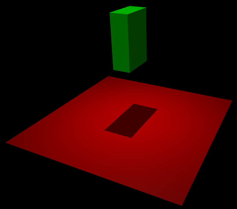
If this model is simulated, the box will fall on the ground. Basic simulation code for the passive dynamics, without rendering, is given below.

hello.c:

#include "mujoco.h"
#include "stdio.h"

char error[1000];
mjModel* m;
mjData* d;

int main(void)
{
   // activate MuJoCo
   mj_activate("mjkey.txt");

   // load model from file and check for errors
   m = mj_loadXML("hello.xml", NULL, error, 1000);
   if( !m )
   {
      printf("%s\n", error);
      return 1;
   }

   // make data corresponding to model
   d = mj_makeData(m);

   // run simulation for 10 seconds
   while( d->time<10 )
      mj_step(m, d);

   // free model and data, deactivate
   mj_deleteData(d);
   mj_deleteModel(m);
   mj_deactivate();

   return 0;
}

This is technically a C file, but it is also a legitimate C++ file. Indeed the MuJoCo API is compatible with both C and C++. Normally user code would be written in C++ because it adds convenience, and does not sacrifice efficiency because the computational bottlenecks are in the simulator which is already highly optimized.

The function mj_step is the top-level function which advances the simulation state by one time step. This example of course is just a passive dynamical system. Things get more interesting when the user specifies controls or applies forces and starts interacting with the system.

Next we provide a more elaborate example illustrating several features of MJCF.

example.xml:

<mujoco model="example">
    <compiler coordinate="global"/>
    <default>
        <geom rgba=".8 .6 .4 1"/>
    </default>
    <asset>
        <texture type="skybox" builtin="gradient" rgb1="1 1 1" rgb2=".6 .8 1" 
                 width="256" height="256"/>
    </asset>
    <worldbody>
        <light pos="0 1 1" dir="0 -1 -1" diffuse="1 1 1"/>
        <body>
            <geom type="capsule" fromto="0 0 1  0 0 0.6" size="0.06"/>
            <joint type="ball" pos="0 0 1"/>
            <body>
                <geom type="capsule" fromto="0 0 0.6  0.3 0 0.6" size="0.04"/>
                <joint type="hinge" pos="0 0 0.6" axis="0 1 0"/>      
                <joint type="hinge" pos="0 0 0.6" axis="1 0 0"/>      
                <body>
                    <geom type="ellipsoid" pos="0.4 0 0.6" size="0.1 0.08 0.02"/>
                    <site name="end1" pos="0.5 0 0.6" type="sphere" size="0.01"/>
                    <joint type="hinge" pos="0.3 0 0.6" axis="0 1 0"/>        
                    <joint type="hinge" pos="0.3 0 0.6" axis="0 0 1"/>        
                </body>
            </body>
        </body>
        <body>
            <geom type="cylinder" fromto="0.5 0 0.2  0.5 0 0" size="0.07"/>
            <site name="end2" pos="0.5 0 0.2" type="sphere" size="0.01"/>
            <joint type="free"/>
        </body>
    </worldbody>
    <tendon>
        <spatial limited="true" range="0 0.6" width="0.005">
            <site site="end1"/>
            <site site="end2"/>
        </spatial>
    </tendon>
</mujoco>

This model is a 7 degree-of-freedom arm "holding" a string with a cylinder attached at the other end. The string is implemented as a tendon with length limits. There is ball joint at the shoulder and pairs of hinge joints at the elbow and wrist. The box inside the cylinder indicates a free "joint". The outer body element in the XML is the required worldbody. Note that using multiple joints between two bodies does not require creating dummy bodies. The MJCF file contains the minimum information needed to specify the model. Capsules are defined by "connecting" points in space - in which case only the radius of the capsule is needed. The positions and orientations of body frames are inferred from the geoms belonging to them. Inertial properties are inferred from the geom shape under a uniform density assumption. The two sites are named because the tendon definition needs to reference them, but nothing else is named. Joint axes are defined only for the hinge joints but not the ball joint. Collision rules are defined automatically. Friction properties, gravity, simulation time step etc. are set to their defaults. The default geom color specified at the top applies to all geoms. Apart from saving the compiled model in the binary MJB format, we can save it as MJCF or as human-readable text; see example_saved.xml and example_saved.txt respectively. The XML version is similar to the original, while the text version contains all information from mjModel. Comparing the text version to the XML version reveals how much work the model compiler did for us.

Performance

Here we illustrate the performance of MuJoCo and compare it to alternative simulators. The details can be found in the sections below. The take-away points in each section can be summarized as follows:

Performance of MuJoCo 2.0
MuJoCo 2.0 has code improvements making it 20% to 80% faster than MuJoCo 1.5 depending on the model. On an Intel i9-7900X processor, all-core performance is 300,000 samples per second on a 3D humanoid model, and 7,000 samples per second on a system with 1000 particles.

Convergence of different constraint solvers
MuJoCo has a direct Newton solver with second-order convergence, in addition to Projected Gauss Seidel and Conjugate Gradient solvers with first-order convergence. In more challenging models, Newton can compute contact forces accurate to numerical precision in 5 iterations, while Gauss Seidel (used in every other engine) can take thousands of iterations to do the same.

Comparison to Flex
On a 3D humanoid model, MuJoCo on CPU is substantially faster than Flex om GPU with the GPU fully saturated, although the comparison is indirect and the setting is not identical. On particle simulations Flex will most likely win, while intermediate cases involving flexible objects remain to be compared. MuJoCo 2.0 allows full interaction between flexible objects and multi-joint dynamics.

Importance of model design
Benchmarks using poorly designed MuJoCo models can create the impression of lower performance, but this can be resolved by designing the models better. MuJoCo 2.0 has an optimizing model compiler which can improve the model design automatically, yielding 50% speedup in some cases. But it cannot always do it, just like a C++ compiler cannot re-write poorly written code.

Comparison to SD/FAST
On multi-joint systems without contacts or other constraints, MuJoCo performs similarly to SD/FAST, even though SD/FAST generates model-specific C code and has more limited functionality.

Comparison to Bullet, Havoc, ODE and PhysX
Compared to gaming engines, MuJoCo is both faster and more accurate in multi-joint dynamics simulations relevant to robotics and control. In simulations with many floating bodies, MuJoCo 2.0 has code improvements yielding similar speed as gaming engines, and scaling linearly with the number of bodies.

Performance of MuJoCo 2.0

MuJoCo 2.0 has multiple code optimizations which increase simulation speed compared to MuJoCo 1.5, by 20% for smaller models and 40% to 80% for larger models. It can also simulate composite flexible objects, modeled as large collections of rigid bodies coupled with soft constraints (where speed is particularly important). Here we provide test results obtained with the code sample 'speedtest' on several models in the software distribution.



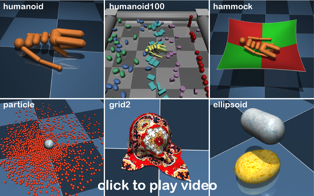
The table below shows size statistics for each model, and number of evaluations per second in one thread and in 20 threads. The latter is more representative of applications that rely on parallel sampling. We tested on a i9-7900X processor, Windows 10, no over-clocking. This processor has 10 physical cores, and we have observed that maximum throughput is achieved when the number of parallel simulations equals the number of logical cores. The simulation time step in all cases is 5 ms. The last column shows the speedup of MuJoCo 2.0 compared to MuJoCo 1.5. The large speedup on the ellipsoid model is because the new soft objects exposed a particular inefficiency in the collision pruning mechanism, which was fixed in MuJoCo 2.0.

model	bodies	DOFs	constraints	evals / s 1 thread	evals / s 20 threads	speedup in version 2.0
humanoid	14	27	56	28,100	300,800	20 %
humanoid100	114	627	1041	1,600	17,100	38 %
hammock	113	312	264	3,340	40,400	83 %
particle	1002	3000	998	880	7,150	52 %
grid2	83	243	475	1,800	19,350	30 %
ellipsoid	213	216	670	3,050	31,600	675 %

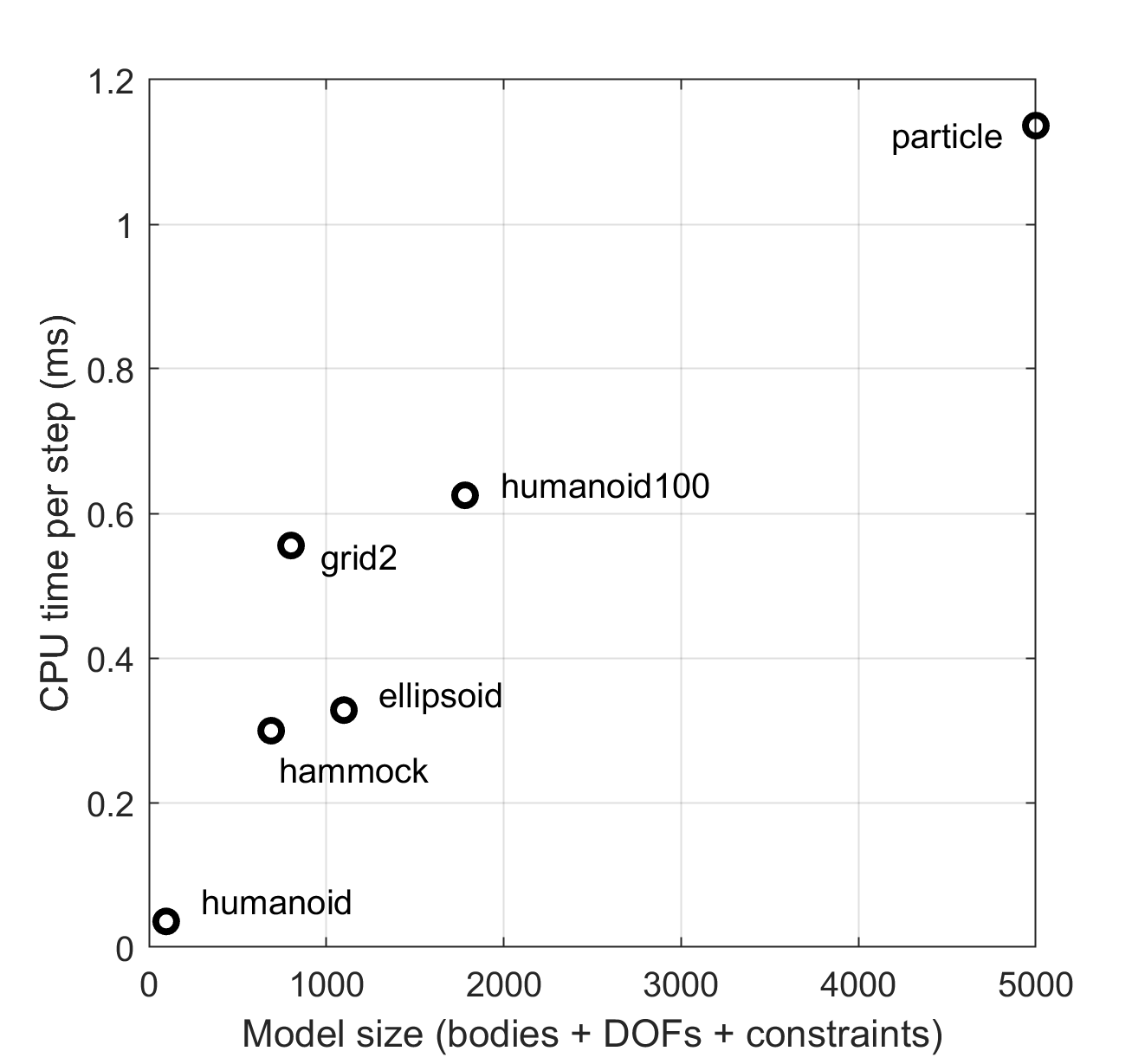
We see that performance with all cores fully loaded is roughly 10x compared to single-thread performance, which is to be expected but also shows that there are no bottlenecks in scaling to multiple threads. Larger models of course take longer to simulate. The plot below shows single-thread performance as a function of model size, where size is defined as (#bodies + #DOFs + #constraints). We have plotted performance as CPU time per step (the inverse of the above numbers) to make the point that scaling is roughly linear. This is because MuJoCo exploits sparsity.

Convergence of different constraint solvers

MuJoCo is based on a unique formulation of contact dynamics which can be solved by a direct Newton method. Its quadratic convergence enables it to compute contact forces accurate to numerical precision, usually in less than 5 iterations even without warm-start. Of course the per-iteration cost is higher than first-order methods such as Gauss-Seidel, but the trade-off is favorable in most models, which is why it is the default solver. For situations where lower accuracy has to be accepted in the name of speed, MuJoCo also offers a Projected Gauss-Seidel (PGS) method similar to other engines, and a Conjugate Gradient (CG) method unique to MuJoCo.

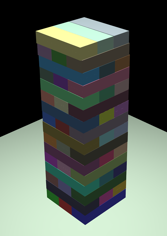
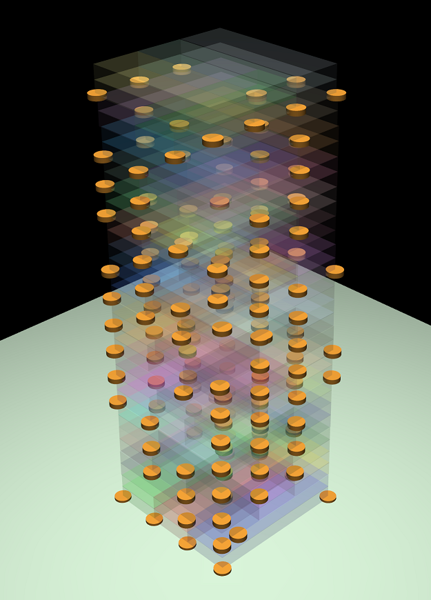
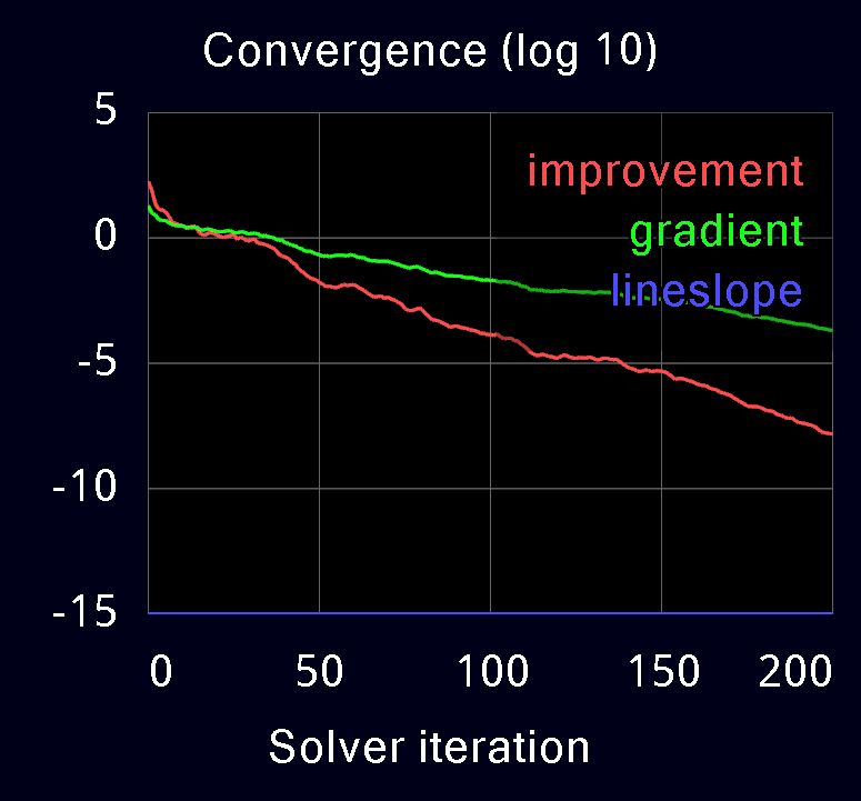
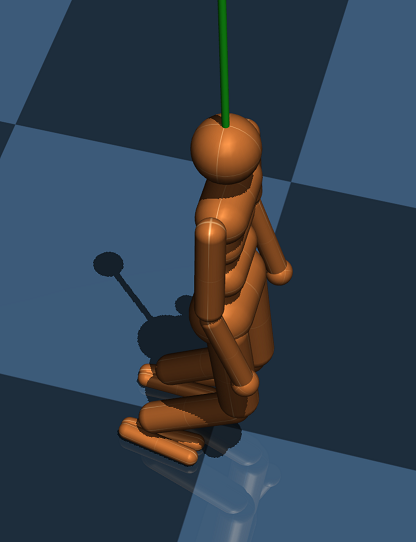
Here we illustrate the convergence of the three solvers, on the humanoid model used earlier and on a more challenging model which is a Jenga tower. It is actually possible to play Jenga in MuJoCo. This requires the blocks to be slightly asymmetric, otherwise friction makes the entire tower fall whenever a block is pulled. The asymmetry causes an irregular pattern of active contacts (see transparent image below) which in turn makes it difficult to compute contact forces accurately.



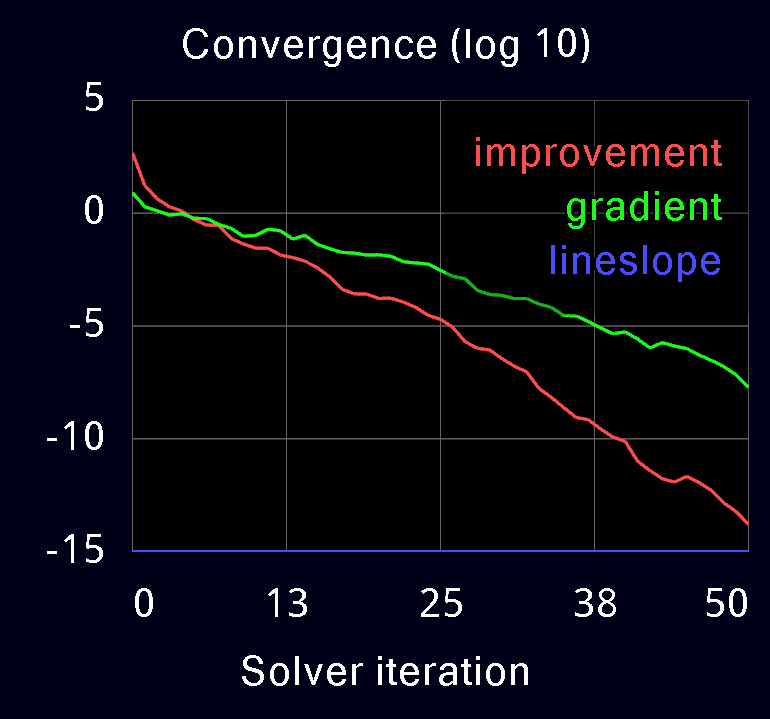
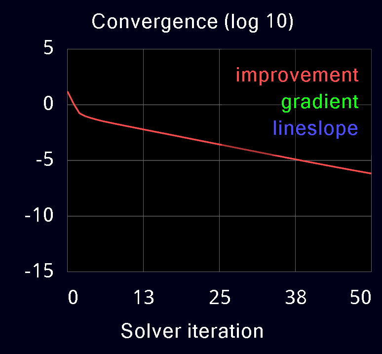
The following plots are obtained from MuJoCo's built-in profiler. Warm-starts are disabled in all cases. The red curve is the reduction in residual at each iteration of the solver. The green and blue curves are the residual gradient and the residual slope in linesearch; these are not available in PGS.

	Newton	Conjugate Gradient	Projected Gauss Seidel
Humanoid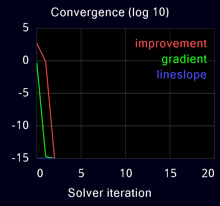
Jenga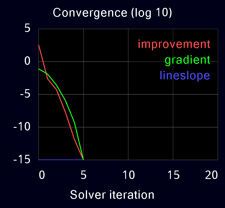

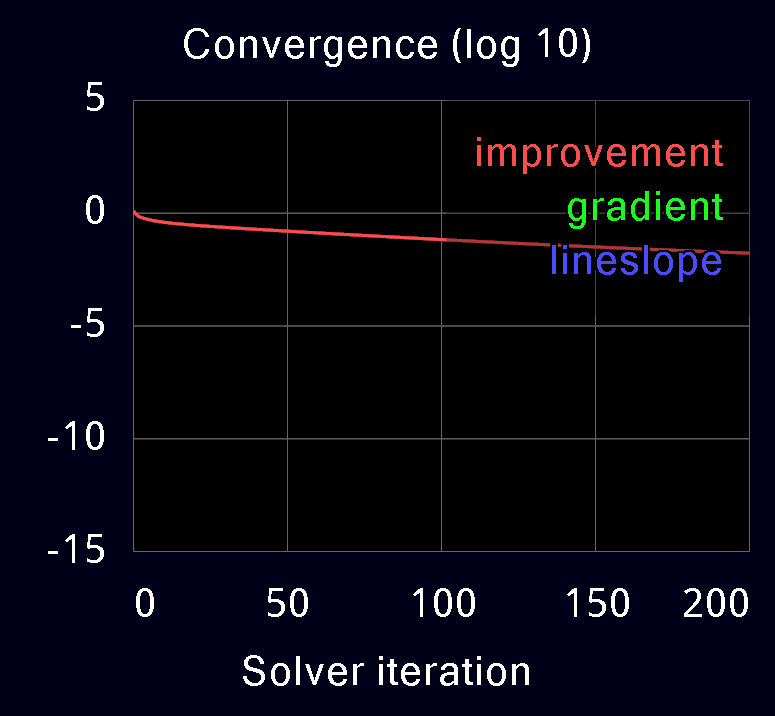We see the quadratic convergence of Newton and the linear convergence of CG and PGS. CG has higher slope than PGS and converges faster, with similar per-iteration cost. Note the poor performance of PGS on the Jenga test. Even after 1000 iterations (not shown) the change-in-residual of PGS is still 1e-4, while CG reaches the tolerance of 1e-15 in about 300 iterations, and Newton reaches it in 5 iterations. We have observed similar behavior in models where heavy bodies and light bodies interact through contact; this occurs for example when the fingertips of a robotic hand try to grasp a heavy object.

Comparison to Flex

Flex is a new simulator from NVidia. It represents the system as a collection of particles and imposes soft constraints among them, similar in spirit to the way MuJoCo 2.0 represents flexible objects. In fact MuJoCo has always supported soft constraints so it could have simulated flexible objects 8 years earlier, but those models are too big to write by hand, and we did not implement an automated model generator earlier. Flex also has a separate subsystem for rigid body dynamics. As explained in the Overview chapter of the documentation, our previous attempts to port MuJoCo to GPUs were not competitive with the CPU version. So it is interesting to compare to Flex. In a recent presentation from NVidia at SIMPAR 2018 it was shown that Flex can simulate around 1000 orange MuJoCo humanoids in realtime on a GTX 1080. We will use this number as a reference for an indirect comparison.

How many humanoids can MuJoCo simulate on a CPU? The NVidia tests were done in the context of locomotion where the number of contacts is smaller compared to lying on the floor, but at the same time the solution changes so warm-starting is less useful. Therefore we added an elastic string to keep our humanoid upright, and made the string anchor point move around to simulate dynamic conditions. We set the simulation timestep to 20ms. This is large, however a key advantage of MuJoCo's contact model is that it can be used with large timesteps even in tasks that require accuracy; see Comparison to Bullet, Havoc, ODE and PhysX below. Flex uses a timestep of around 8ms in this case; whether it can be made larger remains to be seen.



On the same i9-7900X processor as before, we measured 33,800 evaluations per second in a single thread and 387,700 in 20 threads. Given the 20ms simulation timestep, this means that a single core of an Intel CPU can simulate 675 humanoids in realtime, and all 10 cores can simulate 7755 humanoids in realtime. This is substantially faster than Flex on the GPU, even though the GPU has roughly double the transistor count and power consumption. We should emphasize here that the comparison we are making is indirect. The timestep is different, as already discussed. Another difference is that the Flex example involves a large scene with many humanoids, which rarely contact each other but nevertheless contact pruning becomes more expensive. On the other hand, it is possible that large scenes are needed to mask latencies - in which case the GPU would be trading latency for collision overhead. The latter point remains to be clarified, but what we do know is that MuJoCo users can obtain maximum performance without having to create large scenes.

What about particle simulations? We have no doubt that the GPU will win by a large margin in that case. There is a continuum of physical systems, from decoupled systems where GPUs win, to strongly coupled systems where CPUs win. Somewhere in the middle of this continuum lies a gray zone which is just beginning to be explored in physics simulation. Systems in that zone have large numbers of elements coupled with soft yet relatively strong constraints, which may or may not be tractable with the first-order Gauss-Seidel methods used on GPUs (note that MuJoCo has a direct Newton method which is essentially exact). The flexible objects introduced in Flex as well as MuJoCo 2.0 likely live in that zone, and so a side-by-side comparison on such models will be very interesting but remains to be done.

There are several additional considerations regarding CPU vs. GPU, orthogonal to the comparison between MuJoCo and Flex. First, computational research often relies on cloud computing where GPU instances remain expensive. Second, using GPUs involves PCI latencies and added software complexity. Third, during development users usually need a single simulation to run as fast as possible - so as to enable interactive design of models and algorithms. Computing resources are expensive, but salaries are even more expensive.

Importance of model design

MuJoCo has a powerful modeling language, with many element types that can interact in complex ways. This enables users to create elaborate models and customize them as desired, but can also lead to models that do not map well to the MuJoCo framework and have reduced performance or unexpected behavior. The online documentation contains a lot of information on how to design good models.

A common mistake is to create dummy bodies for every joint, sensor or spatial location of interest. A MuJoCo body is not the same thing as a body in a gaming engine. Instead, it is a container for other elements. To help users avoid this mistake, MuJoCo 2.0 introduced the "fusestatic" compiler optimization where bodies that cannot move relative to their parent are fused with the parent. We illustrate the effect on the Anymal model used at ETH Zurich (thanks to Jemin Hwangbo for providing the URDF).



We import this URDF in MuJoCo 2.0 with and without the fusestatic optimization, and test simulator performance. Without fusestatic, we obtain 182,000 samples per second (single thread). With fusestatic the result is 279,000 samples per second. So fusing the dummy bodies (without changing the physics in any way) results in 53% speedup. If we add a floating joint at the base, we get 231,000 samples per second. This is slightly faster than the results for RaiSim from ETH Zurich in their energy test.

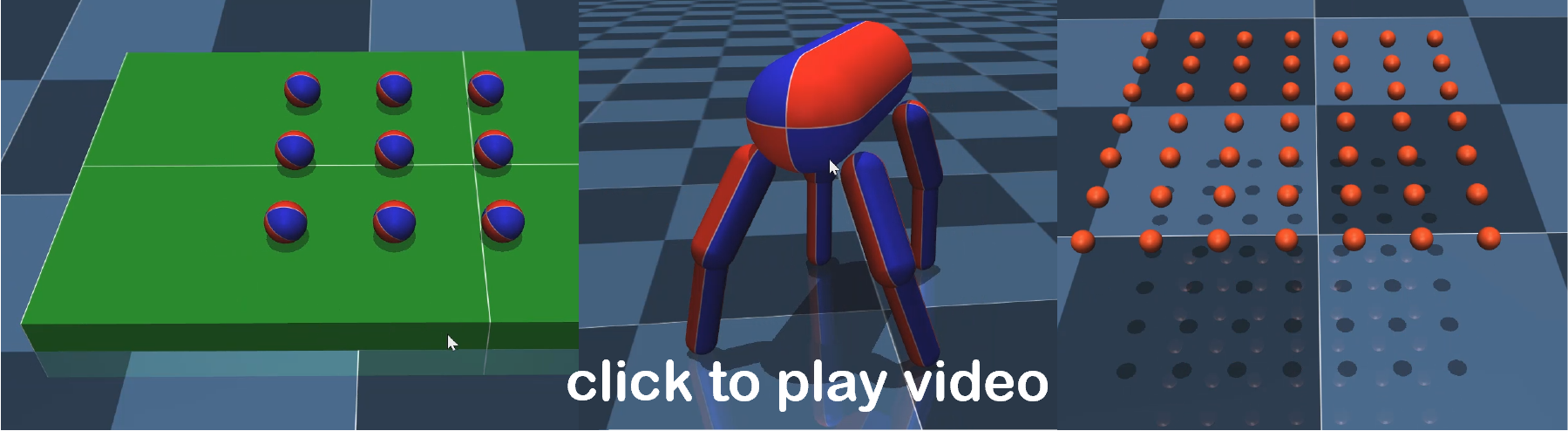
The above mentioned test suite makes other claims about MuJoCo, some of which are accurate - in particular the absence of proper restitution in earlier versions (now present in MuJoCo 2.0). Others are based on arbitrary definitions of accuracy - for example using penetration to compare a soft and a hard model (of course the soft model allows penetrations, that is what it is designed to do, and indeed many objects in the world are somewhat soft). Yet others are based on poorly designed MuJoCo models. For example, balls rolling on a horizontal platform will jump a bit if you make the platform slip on the ground (what this buys you is a convex, smooth and invertible contact model with benefits not found elsewhere). But instead of making the platform slip, one can model the platform as being mounted on a sliding joint, which is the desired effect anyway. Then the contact jumps disappear and the balls roll perfectly, as shown in the video below. Furthermore they stop when the platform stops - which is a known property of this physical system and can be used for accuracy testing. Another example is using MuJoCo's noslip solver to make a quadruped model stand. The noslip solver makes MuJoCo similar to traditional engines based on LCP formulations and Gauss-Seidel methods, and destroys some of the unique properties of MuJoCo's contact model, and is rarely needed. Instead one can use the impratio option and elliptic friction cones to reduce slip, to the point where any remaining slip becomes irrelevant in practice. This is illustrated in the video below, together with the new restitution functionality.

Comparison to SD/FAST

Data from:   MuJoCo: A physics engine for model-based control
E. Todorov, T. Erez, and Y. Tassa (2012). International Conference on Intelligent Robots and Systems

SD/FAST is a cross-compiler that generates model-specific C code for simulating multi-joint dynamics. Even though it has not been updated in nearly 20 years, it has remained the gold standard in many ways. This is partly because model-specific C code is hard to compete with, and partly because at the time people used to calculate the exact number of floating point operations and optimize numerical performance aggressively. This is why when we began working on MuJoCo we did not aim to outperform SD/FAST, but rather to come close to it in terms of multi-joint dynamics while adding contact dynamics and other important features.

We compared MuJoCo and SD/FAST on four model systems: isolated bodies, a chain, a hand, and a humanoid model. To our pleasant surprise, the outcome was a tie: MuJoCo was faster on some tests while SD/FAST was faster on others. The table below shows the number of evaluations per second, rounded to 1000, on one core of a now-outdated Intel processor (average over X9650, X5570, i7 940, X5860).

Model (DOF)	SD/FAST eval/s	MuJoCo eval/s
Isolated (34)	122,000	151,000
Chain (31)	128,000	103,000
Hand (32)	89,000	101,000
Humanoid (29)	130,000	123,000

Each evaluation was performed at a randomly-generated state (same for both engines), and included computation of the joint-space inertia matrix and the vector of Coriolis, centripetal and gravitational forces. Once these quantities are available, physics simulation comes down to solving a linear system. Note that we did not use the O(N) solver in SD/FAST, because that solver does not compute the inertia matrix which is essential for simulating contact dynamics. Instead we used the solver which implements similar algorithms to those used in MuJoCo.

Comparison to Bullet, Havoc, ODE and PhysX

Data from:   Simulation tools for model-based robotics: Comparison of Bullet, Havok, MuJoCo, ODE and PhysX
T. Erez, Y. Tassa and E. Todorov (2015). International Conference on Robotics and Automation

Bullet, Havoc, ODE and PhysX are among the most popular engines used today for gaming, animation and multi-body dynamics simulation. They come from the tradition of the now-retired MathEngine, and represent the system in Cartesian coordinates (with 6 DOFs per body) while joints are represented as equality constraints imposed numerically. This is natural for systems involving many floating bodies. But for robotic and biomechanical systems where the DOF-to-body ratio is typically close to 1, a joint coordinate representation (as in MuJoCo and SD/FAST) is more efficient computationally, and also more accurate - because the joints cannot dislocate and thus the engine does not have to fix constraint violations at each step.

Our empirical results are consistent with the above reasoning. For multi-joint systems relevant to robotics and biomechanics MuJoCo is the fastest, while for systems composed of many floating bodies MuJoCo is the slowest and ODE is the fastest. Simulation speed however is not the most relevant measure of performance. Speed can always be increased by using a larger timestep, but this comes at the expense of accuracy and stability. So the more relevant measure is the speed-accuracy trade-off of each engine. We define accuracy by running the simulation with a very small timestep (0.016 ms) where all engines should be very accurate, and then measuring the deviations from the engine-specific reference as the timestep increases. We find that even for systems that are better suited for gaming engines, MuJoCo is the fastest at a fixed accuracy level and the most accurate at a fixed speed level. This is because it can use much larger timesteps without loosing accuracy.

Note that the above measure of accuracy is with respect to an engine-specific reference and not an analytical benchmark. This is because we want to have a measure that can be applied to complex systems where analytical results are not available. As a result, an engine can simulate "physics" that deviate from reality without being penalized. For example, both Havoc and PhysX ignore Coriolis forces. But since they do that for all timesteps, our accuracy measure (which really reflects self-consistency) does not penalize them.

The figure below shows four test systems we simulated in each engine (left column), raw speed (middle column), and speed-accuracy trade-off (right column). MuJoCo has two flavors depending on the integrator being used: semi-implicit Euler vs. 4th-order Runge Kutta. For one of the test systems (planar chain) we were also able to use the new version of Bullet (labeled BulletMB) which operates in joint coordinates; for the other systems it seemed to need more work before it can be used reliably. PhysX also has a version aimed at simulating multi-joint systems, but it does not use joint coordinates; instead it relies on the underlying Cartesian representation and has similar behavior as the standard version.



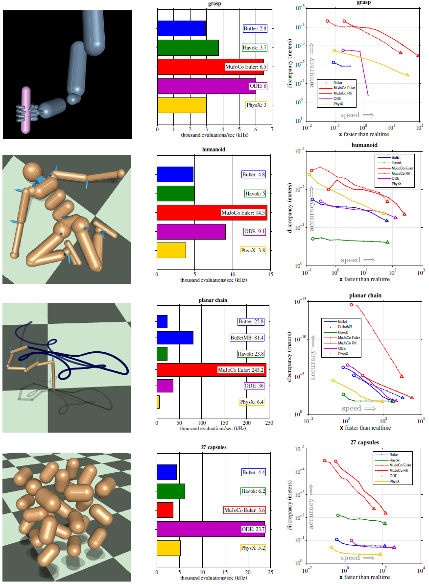
Some of the speed-accuracy curves are incomplete because when a given engine diverges at a given timestep we cannot obtain a measurement. The hand grasping an object was the most challenging test system, and is also very relevant to robotics. To measure the maximum timestep at which each engine could simulate this system without dropping the object, we started at timestep 1/64 ms and increased it by factor of 2 until the object was dropped. The table below shows the last successful timestep for each engine. Note the order-of-magnitude difference between MuJoCo and the best-performing gaming engine in this test (PhysX).

Engine	Max timestep
Bullet	0.031 ms
MuJoCo	16 ms
ODE	0.25 ms
PhysX	2 ms

Model elements

This section provides brief descriptions of all elements that can be included in a MuJoCo model. Later we explain in more detail the underlying computations, the way elements are specified in MJCF, and their representation in mjModel.

Options

Each model has three sets of options listed below. They are always included. If their values are not specified in the XML file, default values are used. The options are designed such that the user can change their values before each simulation time step. Within a time step however none of the options should be changed.

mjOption

This structure contains all options that affect the physics simulation. It is used to select algorithms and set their parameters, enable and disable different portions of the simulation pipeline, and adjust system-level physical properties such as gravity.

mjVisual

This structure contains all visualization options. There are additional OpenGL rendering options, but these are session-dependent and are not part of the model.

mjStatistic

This structure contains statistics about the model which are computed by the compiler: average body mass, spatial extent of the model etc. It is included for information purposes, and also because the visualizer uses it for automatic scaling.

Assets

Assets are not in themselves model elements. Model elements can reference them, in which case the asset somehow changes the properties of the referencing element. One asset can be referenced by multiple model elements. Since the sole purpose of including an asset is to reference it, and referencing can only be done by name, every asset has a name (which may be inferred from a file name when applicable). In contrast, the names of regular elements are often left undefined.

Mesh

MuJoCo can load triangulated meshes from binary STL files. Software such as MeshLab can be used to convert from other formats. While any collection of triangles can be loaded and visualized as a mesh, the collision detector works with the convex hull. There are compile-time options for scaling the mesh, as well as fitting a primitive geometric shape to it. The mesh can also be used to automatically infer inertial properties - by treating it as a union of triangular pyramids and combining their masses and inertias. Note that the STL format does not support color; some software packages write color information in unused fields but this is not consistent. Instead the mesh is colored using the material properties of the referencing geom. In contrast, all spatial properties are determined by the mesh data and the size parameters of the referencing geom are ignored. As of MuJoCo 2.0, meshes can also be loaded from custom binary files that can additionally specify normals and texture coordinates. Meshes can also be embedded directly in the XML.

Skin

Skinned meshes (or skins) are meshes whose shape can deform at runtime. Their vertices are attached to rigid bodies (called bones in this context) and each vertex can belong to multiple bones, resulting in smooth deformations of the skin. Skins are purely visualization objects and do not affect the physics, but nevertheless they can enhance visual realism significantly. Skins can be loaded from custom binary files, or emebdded directly in the XML, similar to meshes. When generating composite flexible objects automatically, the model compiler also generates skins for these objects.

Height field

Height fields can be loaded from PNG files (converted to gray-scale internally) or from files in a custom binary format described later. A height field is a rectangular grid of elevation data. The compiler normalizes the data to the range [0-1]. The actual spatial extent of the height field is then determined by the size parameters of the referencing geom. Height fields can only be referenced from geoms that are attached to the world body. For rendering and collision detection purposes the grid rectangles are automatically triangulated, thus the height field is treated as a union of triangular prisms. Collision detection with such a composite object can in principle generate a large number of contact points for a single geom pair. If that happens, only the first 16 contact points are kept. The rationale is that height fields should be used to model terrain maps whose spatial features are large compared to the other objects in the simulation - and so the number of contacts will be small for well-designed models.

Texture

Textures can be loaded from PNG files or synthesized by the compiler based on user-defined procedural parameters. There is also the option to leave the texture empty at model creation time and change it later at runtime - so as to render video in a MuJoCo simulation, or create other dynamic effects. The visualizer supports two types of texture mapping: 2D and cube. 2D mapping is useful for planes and height fields. Cube mapping is useful for "shrink-wrapping" textures around 3D objects without having to specify texture coordinates. It is also used to create a skybox. The six sides of a cube maps can be loaded from separate image files, or from one composite image file, or generated by repeating the same image. Unlike all other assets which are referenced directly from model elements, textures can only be referenced from another asset (namely material) which is then referenced from model elements.

Material

Materials are used to control the appearance of geoms, sites and tendons. This is done by referencing the material from the corresponding model element. Appearance includes texture mapping as well as other properties that interact with OpenGL lights below: RGBA, specularity, shininess, emission. Materials can also be used to make objects reflective. Currently reflections are rendered only on planes and on the Z+ faces of boxes. Note that model elements can also have their local RGBA parameter for setting color. If both material and local RGBA are specified, the local definition has precedence.

Kinematic tree

MuJoCo simulates the dynamics of a collection of rigid bodies whose motion is usually constrained. The system state is represented in joint coordinates and the bodies are explicitly organized into kinematic trees. Each body except for the top-level "world" body has a unique parent. Kinematic loops are not allowed; if loop joints are needed they should be modeled with equality constraints. Thus the backbone of a MuJoCo model is one or several kinematic trees formed by nested body definitions; an isolated floating body counts as a tree. Several other elements listed below are defined within a body and belong to that body. This is in contrast with the stand-alone elements listed later which cannot be associated with a single body.

Body

Bodies have mass and inertial properties but do not have any geometric properties. Instead geometric shapes (or geoms) are attached to the bodies. Each body has two coordinate frames: the frame used to define it as well as to position other elements relative to it, and an inertial frame centered at the body's center of mass and aligned with its principal axes of inertia. The body inertia matrix is therefore diagonal in this frame. At each time step MuJoCo computes the forward kinematics recursively, yielding all body positions and orientations in global Cartesian coordinates. This provides the basis for all subsequent computations.

Joint

Joints are defined within bodies. They create motion degrees of freedom (DOFs) between the body and its parent. In the absence of joints the body is welded to its parent. This is the opposite of gaming engines which use over-complete Cartesian coordinates, where joints remove DOFs instead of adding them. There are four types of joints: ball, slide, hinge, and a free "joint" which creates floating bodies. A single body can have multiple joints. In this way composite joints are created automatically, without having to define dummy bodies. The orientation components of ball and free joints are represented as unit quaternions, and all computations in MuJoCo respect the properties of quaternions.

DOF

Degrees of freedom are closely related to joints, but are not in one-to-one correspondence because ball and free joints have multiple DOFs. Think of joints as specifying positional information, and of DOFs as specifying velocity and force information. More formally, the joint positions are coordinates over the configuration manifold of the system, while the joint velocities are coordinates over the tangent space to this manifold at the current position. DOFs have velocity-related properties such as friction loss, damping, armature inertia. All generalized forces acting on the system are expressed in the space of DOFs. In contrast, joints have position-related properties such as limits and spring stiffness. DOFs are not specified directly by the user. Instead they are created by the compiler given the joints.

Geom

Geoms are 3D shapes rigidly attached to the bodies. Multiple geoms can be attached to the same body. This is particularly useful in light of the fact that MuJoCo only supports convex geom-geom collisions, and the only way to create non-convex objects is to represent them as a union of convex geoms. Apart from collision detection and subsequent computation of contact forces, geoms are used for rendering, as well as automatic inference of body masses and inertias when the latter are omitted. MuJoCo supports several primitive geometric shapes: plane, sphere, capsule, ellipsoid, cylinder, box. A geom can also be a mesh or a height field; this is done by referencing the corresponding asset. Geoms have a number of material properties that affect the simulation and visualization.

Site

Sites are essentially light geoms. They represent locations of interest within the body frame. Sites do not participate in collision detection or automated computation of inertial properties, however they can be used to specify the spatial properties of other objects: sensors, tendon routing, slider-crank endpoints.

Camera

Multiple cameras can be defined in a model. There is always a default camera which the user can freely move with the mouse in the interactive visualizer. However it is often convenient to define additional cameras that are either fixed to the world, or are attached to one of the bodies and move with it. In addition to the camera position and orientation, the user can adjust the field of view and the inter-pupilary distance for stereoscopic rendering, as well as create oblique projections needed for stereoscopic virtual environments.

Light

Lights can be fixed to the world body or attached to moving bodies. The visualizer provides access to the full lighting model in OpenGL (fixed function) including ambient, diffuse and specular components, attenuation and cutoff, positional and directional lighting, fog. Lights, or rather the objects illuminated by them, can also cast shadows. However, similar to material reflections, each shadow-casting light adds one rendering pass so this feature should be used with caution. Documenting the lighting model in detail is beyond the scope of this chapter; see OpenGL documentation instead. Note that in addition to lights defined by the user in the kinematic tree, there is a default headlight that moves with the camera. Its properties are adjusted through the mjVisual options.

Stand-alone elements

Here we describe the model elements which do not belong to an individual body, and therefore are defined outside the kinematic tree.

Reference pose

The reference pose is a vector of joint positions stored in mjModel.qpos0. It corresponds to the numeric values of the joints when the model is in its initial configuration. In our earlier example the elbow was created in a bent configuration at 90 deg angle. But MuJoCo does not know what an elbow is, and so by default it treats this joint configuration as having numeric value of 0. We can override the default behavior and specify that the initial configuration corresponds to 90 deg, using the ref attribute of joint. The reference values of all joints are assembled into the vector mjModel.qpos0. Whenever the simulation is reset, the joint configuration mjData.qpos is set to mjModel.qpos0. At runtime the joint position vector is interpreted relative to the reference pose. In particular, the amount of spatial transformation applied by the joints is mjData.qpos - mjModel.qpos0. This transformation is in addition to the parent-child translation and rotation offsets stored in the body elements of mjModel. The ref attribute only applies to scalar joints (slide and hinge). For ball joints, the quaternion saved in mjModel.qpos0 is always (1,0,0,0) which corresponds to the null rotation. For free joints, the global 3D position and quaternion of the floating body are saved in mjModel.qpos0.

Spring reference pose

This is the pose in which all joint and tendon springs achieve their restring length. Spring forces are generated when the joint configuration deviates from the spring reference pose, and are linear in the amount of deviation. The spring reference pose is saved in mjModel.qpos_spring. For slide and hinge joints, the spring reference is specified with the attribute springref. For ball and free joints, the spring reference corresponds to the initial model configuration.

Tendon

Tendons are scalar length elements that can be used for actuation, imposing limits and equality constraints, or creating spring-dampers and friction loss. There are two types of tendons: fixed and spatial. Fixed tendons are linear combinations of (scalar) joint positions. They are useful for modeling mechanical coupling. Spatial tendons are defined as the shortest path that passes through a sequence of specified sites (or via-points) or wraps around specified geoms. Only spheres and cylinders are supported as wrapping geoms, and cylinders are treated as having infinite length for wrapping purposes. To avoid abrupt jumps of the tendon from one side of the wrapping geom to the other, the user can also specify the preferred side. If there are multiple wrapping geoms in the tendon path they must be separated by sites, so as to avoid the need for an iterative solver. Spatial tendons can also be split into multiple branches using pulleys.

Actuator

MuJoCo provides a flexible actuator model, with three components that can be specified independently. Together they determine how the actuator works. Common actuator types are obtained by specifying these components in a coordinated way. The three components are transmission, activation dynamics, and force generation. The transmission specifies how the actuator is attached to the rest of the system; available types are joint, tendon and slider-crank. The activation dynamics can be used to model internal activation states of pneumatic or hydraulic cylinders as well as biological muscles; using such actuators makes the overall system dynamics 3rd-order. The force generation mechanism determines how the scalar control signal provided as input to the actuator is mapped into a scalar force, which is in turn mapped into a generalized force by the moment arms inferred from the transmission.

Sensor

MuJoCo can generate simulated sensor data which is saved in the global array mjData.sensordata. The result is not used in any internal computations; instead it is provided because the user presumably needs it for custom computation or data analysis. Available sensor types include touch sensors, inertial measurement units (IMUs), force-torque sensors, joint and tendon position and velocity sensors, actuator position, velocity and force sensors, motion capture marker positions and quaternions, and magnetometers. Some of these require extra computation, while others are copied from the corresponding fields of mjData. There is also a user sensor, allowing user code to insert any other quantity of interest in the sensor data array. MuJoCo also has off-screen rendering capabilities, making it straightforward to simulate both color and depth camera sensors. This is not included in the standard sensor model and instead has to be done programmatically, as illustrated in the code sample simulate.cpp.

Equality

Equality constraints can impose additional constraints beyond those already imposed by the kinematic tree structure and the joints/DOFs defined in it. They can be used to create loop joints, or in general model mechanical coupling. The internal forces that enforce these constraints are computed together with all other constraint forces. The available equality constraint types are: connect two bodies at a point (creating a ball joint outside the kinematic tree); weld two bodies together; make two surfaces slide on each other; fix the position of a joint or tendon; couple the positions of two joints or two tendons via a cubic polynomial.

Contact pair

Contact generation in MuJoCo is an elaborate process. Geom pairs that are checked for contact can come from two sources: automated proximity tests and other filters collectively called "dynamic", as well as an explicit list of geom pairs provided in the model. The latter is a separate type of model element. Because a contact involves a combination of two geoms, the explicit specification allows the user to define contact parameters in ways that cannot be done with the dynamic mechanism. It is also useful for fine-tuning the contact model, in particular adding contact pairs that were removed by an aggressive filtering scheme.

Contact exclude

This is the opposite of contact pairs: it specifies pairs of bodies (rather than geoms) which should be excluded from the generation of candidate contact pairs. It is useful for disabling contacts between bodies whose geometry causes an undesirable permanent contact. Note that MuJoCo has other mechanisms for dealing with this situation (in particular geoms cannot collide if they belong to the same body or to a parent and a child body), but sometimes these automated mechanisms are not sufficient and explicit exclusion becomes necessary.

Custom numeric

There are three ways to enter custom numbers in a MuJoCo simulation. First, global numeric fields can be defined in the XML. They have a name and an array of real values. Second, the definition of certain model elements can be extended with element-specific custom arrays. This is done by setting the attributes "nuser_XXX" in the XML element "size". Third, there is the array mjData.userdata which is not used by any MuJoCo computations. The user can store results from custom computations there; recall that everything that changes over time should be stored in mjData and not in mjModel.

Custom text

Custom text fields can be saved in the model. They can be used in custom computations - either to specify keyword commands, or to provide some other textual information. Do not use them for comments though; there is no benefit to saving comments in a compiled model. XML has its own commenting mechanism (ignored by MuJoCo's parser and compiler) which is more suitable.

Custom tuple

Custom tuples are lists of MuJoCo model elements, possibly including other tuples. They are not used by the simulator, but are available for specifying groups of elements that are needed for user code. For example, one can use tuples to define pairs of bodies for custom contact processing.

Keyframe

A keyframe is a snapshot of the simulation state variables. It contains the vectors of joint positions, joint velocities, actuator activations when present, and the simulation time. The model can contain a library of keyframes. They are useful for resetting the state of the system to a point of interest. Note that keyframes are not intended for storing trajectory data in the model; external files should be used for this purpose.

Clarifications

The reader is likely to have experience with other physics simulators and related conventions, as well as general programming practices that are not aligned with MuJoCo. This has the potential to cause confusion. The goal of this section is to preemptively clarify the aspects that are most likely to be confusing; it is somewhere in-between a FAQ and a tutorial on selected topics. We will need to refer to material covered later in the documentation, but nevertheless the text below is as self-contained and introductory as possible.

Not object-oriented

Object-oriented programming is a very useful abstraction, built on top of the more fundamental (and closer-to-hardware) notion of data structures vs. functions that operate on them. An object is a collection of data structures and functions that correspond to one semantic entity, and thereby have stronger dependencies among them than with the rest of the application. The reason we are not using this here is because the dependency structure is such that the natural entity is the entire physics simulator. Instead of objects, we have a small number of data structures and a large number of functions that operate on them.

We still use a type of grouping, but it is different from the object-oriented approach. We separate the model (mjModel) from the data (mjData). These are both data structures. The model contains everything needed to describe the constant properties of the physical system being modeled, while the data contains the time-varying state and the reusable intermediate results of internal computations. All top-level functions expect pointers to mjModel and mjData as arguments. In this way we adoid global variables which pollute the workspace and interfere with multi-threading, but we do so in a way that is different from how object-oriented programming achieves the same effect.

Softness and slip

As we will explain at length in the Computation chapter, MuJoCo is based on a novel mathematical model of the physics of contact and other constraints. This model is inherently soft, in the sense that pushing harder against a constraint will always result in larger acceleration, and so the inverse dynamics can be uniquely defined. This is desirable because it yields a convex optimization problem and enables analyses that rely on inverse dynamics, and furthermore most contacts that we need to model in practice have some softness. However once we allow soft constraints, we are effectively creating a new type of dynamics - namely deformation dynamics - and now we must specify how these dynamics behave. This calls for elaborate parameterization of contacts and other constraints, involving the attributes solref and solimp that can be set per constraints and will be described later.

An often confusing aspect of this soft model is that gradual contact slip cannot be avoided. Similarly, frictional joints will gradually yield under gravity. This is not because the solver is unable to prevent slip, in the sense of reaching the friction cone or friction loss limit, but because it is not trying to prevent slip in the first place. Recall that larger force against a given constraint must result in larger acceleration. If slip were to be fully suppressed, this key property would have to be violated. So if you see gradual slip in your simulation, the intuitive explanation may be that the friction is insufficient, but that is rarely the case in MuJoCo. Instead the solref and solimp parameter vectors need to be adjusted in order to reduce this effect. Increasing constraint impedance (first two elements of solimp) as well as the global mjModel.opt.impratio setting can be particularly effective. Such adjustment often requires smaller time steps to keep the simulation stable, because they make the nonlinear dynamics more difficult to integrate numerically. Slip is also reduced by the Newton solver which is more accurate in general.

For situations where it is desirable to suppress slip completely, there is a second Noslip solver which runs after the main solver. It updates the contact forces in friction dimensions by disregarding constraint softness. When this option is used however, MuJoCo is no longer solving the convex optimization problem it was designed to solve, and the simulation may become less robust resembling a gaming engine. Thus using the Newton solver with elliptic friction cones and large value of impratio is the recommended way of reducing slip.

Types, names, ids

MuJoCo supports a large number of model elements, as summarized earlier. Each element type has a corresponding section in mjModel listing its various properties. For example the joint limit data is in the array

mjtNum* jnt_range;             // joint limits       (njnt x 2)

The size of each array (njnt in this case) is also given in mjModel. The limits of the first joint are included first, followed by the limits of the second joint etc. This ordering reflects the fact that all matrices in MuJoCo have row-major format.

The available element types are defined in mjmodel.h, in the enum type mjtObj. These constants are mostly used internally. One exception are the functions mj_name2id and mj_id2name in the MuJoCo API, which map element names to integer ids and vice versa. These functions take an element type as input. The corresponding functions in the HAPTIX API take a string argument with the type name as input.

Naming model elements in the XML is optional. Two elements of the same type (e.g. two joints) cannot have the same name. Naming is required only when a given element needs to be referenced elsewhere in the model; referencing in the XML can only be done by name. Once the model is compiled, the names are still stored in mjModel for user convenience, although they have no further effect on the simulation. Names are useful for finding the corresponding integer ids, as well as rendering: if you enable joint labels for example, a string will be shown next to each joint (elements with undefined names are labeled as "joint N" where N is the id).

The integer ids of the elements are essential for indexing the MuJoCo data arrays, both in the main API and in the HAPTIX APIs. The ids are 0-based, following the C convention. Suppose we already have mjModel* m. To print the range of a joint named "elbow", do:

int jntid = mj_name2id(m, mjOBJ_JOINT, "elbow");
if( jntid>=0 )
   printf("(%f, %f)\n", m->jnt_range[2*jntid], m->jnt_range[2*jntid+1]); 

If the name is not found the function returns -1, which is why one should always check for id>=0. The same effect can be achieved in the HAPTIX C API as follows. Assuming we already have mjInfo info, do:

int jntid = mj_name2id("joint", "elbow");
if( jntid>=0 )
   printf("(%f, %f)\n", info.jnt_range[2*jntid], info.jnt_range[2*jntid+1]); 

Note the difference between the main API and the HAPTIX API. In the main API we could be working with many different models, so we have to pass a mjModel pointer to mj_name2id. In HAPTIX there is only one model loaded in the simulator. However that model is not kept in the user workspace. The function mj_info provides a summary of the information available in mjModel.

Finally, we could do the same in the HAPTIX MATLAB API as:

jntid = mj_name2id('joint', 'elbow');
if( jntid>=0 )
   fprintf('(%f, %f)\n', info.jnt_range(2*jntid+1), info.jnt_range(2*jntid+2); 

In this case we have to add 1 to the indices, because MATLAB arrays are 1-based, while MuJoCo returns the ids used in the model which are 0-based.

Bodies, geoms, sites

Bodies, geoms and sites are MuJoCo elements which roughly correspond to rigid bodies in the physical world. So why are they separate? For semantic as well as computational reasons explained here.

First the similarities. Bodies, geoms and sites all have spatial frames attached to them (although bodies also have a second frame which is centered at the body center of mass and aligned with the principal axes of inertia). The positions and orientations of these frames are computed at each time step from mjData.qpos via forward kinematics. The results of forward kinematics are availabe in mjData as xpos, xquat and xmat for bodies, geom_xpos and geom_xmat for geoms, site_xpos and site_xmat for sites. HAPTIX users can obtain these quantities by calling mj_get_body, mj_get_geom and mj_get_site respectively.

Now the differences. Bodies are used to construct the kinematic tree and are containers for other elements, including geoms and sites. Bodies have a spatial frame, inertial properties, but no properties related to appearance or collision geometry. This is because such properties do not affect the physics (except for contacts of course, but these are handled separately). If you have seen diagrams of kinematic trees in robotics textbooks, the bodies are usually drawn as amorphous shapes - to make the point that their actual shape is irrelevant to the physics.

Geoms (short for geometric primitive) are used to specify appearance and collision geometry. Each geom belongs to a body and is rigidly attached to that body. Multiple geoms can be attached to the same body. This is particularly useful in light of the fact that MuJoCo's collision detector assumes that all geoms are convex (it internally replaces meshes with their convex hulls if the meshes are not convex). Thus if you want to model a non-convex shape, you have to decompose it into a union of convex geoms and attach all of them to the same body. Geoms can also have mass and inertia in the XML model (or rather material density which is used to compute the mass and ineria), but that is only used to compute the body mass and inertia in the model compiler. In the actual mjModel being simulated geoms do not have inertial properties.

Sites are light geoms. They have the same appearance properties but cannot participate in collisions and cannot be used to infer body masses. On the other hand sites can do things that geoms cannot do: they can specify the volumes of touch sensors, the attachment of IMU sensors, the routing of spatial tendons, the end-points of slider-crank actuators. These are all spatial quantities, and yet they do not correspond to entities that should have mass or collide other entities - which is why the site element was created. Sites can also be used to specify points (or rather frames) of interest to the user.

The following example illustrates the point that multiple sites and geoms can be attached to the same body: two sites and two geoms to one body in this case.

<mujoco>
   <worldbody>
      <body pos="0 0 0">
         <geom type="sphere" size=".1" rgba=".9 .9 .1 1"/>
         <geom type="capsule" pos="0 0 .1" size=".05 .1" rgba=".9 .9 .1 1"/>
         <site type="box" pos="0 -.1 .3" size=".02 .02 .02" rgba=".9 .1 .9 1"/>
         <site type="ellipsoid" pos="0 .1 .3" size=".02 .03 .04" rgba=".9 .1 .9 1"/>
      </body>
   </worldbody>
</mujoco>

This model is rendered by the OpenGL visualizer as:



Note the red box. This is an equivalent-inertia box rendering of the body inertial properties, and is generated by MuJoCo internally. The box is over the geoms but not over the sites. This is because only the geoms were used to (automatically) infer the inertial properties of the body. If we happen to know the latter, we can of course specify them directly. But it is often more convenient to let the model compiler infer these body properties from the geoms attached to it, using the assumption of uniform density (geom density can be specified in the XML; the default is the density of water).

Joint coordinates

One of the key distinctions between MuJoCo and gaming engines (such as ODE, Bullet, Havoc, PhysX) is that MuJoCo operates in generalized or joint coordinates, while gaming engines operate in Cartesian coordinates, although Bullet now supports generalized coordinates. The differences between these two approaches can be summarized as follows:

Joint coordinates:

• Best suited for elaborate kinematic structures such as robots;
• Joints add degrees of freedom among bodies that would be welded together by default;
• Joint constraints are implicit in the representation and cannot be violated;
• The positions and orientations of the simulated bodies are obtained from the generalized coordinates via forward kinematics, and cannot be manipulated directly (except for root bodies).

Cartesian coordinates:

• Best suited for many bodies that bounce off each other, as in molecular dynamics and box stacking;
• Joints remove degrees of freedom among bodies that would be free-floating by default;
• Joint constraints are enforced numerically and can be violated;
• The positions and orientations of the simulated bodies are represented explicitly and can be manipulated directly, although this can introduce further joint constraint violations.

Joint coordinates can be particularly confusing when working with free-floating bodies that are part of a model which also contains kinematic trees. This is clarified below.

Floating objects

When working in joint coordinates, you cannot simply set the position and orientation of an arbitrary body to whatever you want. To achieve that effect you would have to implement some form of inverse kinematics, which computes a (not necessarily unique) set of joint coordinates for which the forward kinematics place the body where you want it to be.

The situation is different for floating bodies, i.e. bodies that are connected to the world with a free joint. The positions and orientations as well as the linear and angular velocities of such bodies are explicitly represented in mjData.qpos and mjData.qvel, and can therefore be manipulated directly. This can be done in two ways. The general approach is to find the addresses in qpos and qvel where the body's data are. Of course qpos and qvel represents joints and not bodies, so you need the corresponding joint addresses. Suppose the body was named "myfloatingbody" in the XML. The necessary addresses can be obtained as:

int bodyid = mj_name2id(m, mjOBJ_BODY, "myfloatingbody");
int qposadr = -1, qveladr = -1;

// make sure we have a floating body: it has a single free joint
if( bodyid>=0 && m->body_jntnum[bodyid]==1 && 
    m->jnt_type[m->body_jntadr[bodyid]]==mjJNT_FREE )
   {
      // extract the addresses from the joint specification
      qposadr = m->jnt_qposadr[m->body_jntadr[bodyid]];
      qveladr = m->jnt_dofadr[m->body_jntadr[bodyid]];
   }

Now if everything went well (i.e. "myfloatingbody" was indeed a floating body), qposadr and qveladr are the addresses in qpos and qvel where the data for our floating body/joint lives. The position data is 7 numbers (3D position followed by unit quaternion) while the velocity data is 6 numbers (3D linear velocity followed by 3D angular velocity). These numbers can now be set to the desired pose and velocity of the body.

The same can be achieved in the HAPTIX API, however a somewhat different approach is needed because mjModel is not available to the HAPTIX user; instead the user can obtain a summary data structure called mjInfo. To find our body, we will scan the list jnt_bodyid and look for a free joint attached to our body (this can also be done in the main API of course):

mjInfo info;
mj_info(&info);
int bodyid = mj_name2id("body", "myfloatingbody");
int qposadr = -1, qveladr = -1;

// scan list of joints for matching bodyid and type
for( int i=0; i<info.njnt; i++ )
   if( info.jnt_bodyid[i]==bodyid && info.jnt_type[i]==mjJNT_FREE )
   {
      qposadr = info.jnt_qposadr[i];
      qveladr = info.jnt_dofadr[i];
      break;
   }

All this is doable but somewhat roundabout. Since this is likely to be a common operation, we have introduced utility functions in the HAPTIX API that do all the necessary indexing internally and get/set the pose and velocity of a floating body. An added benefit is that one can get/set only part of the state vector, instead of sending the entire state vector over the socket connection. These functions are mj_get_floatbody and mj_set_floatbody. We can now for example move a floating body by 1cm along the x-axis as:

int bodyid = mj_name2id("body", "myfloatingbody");
mjFloatBody fbody;
mj_get_floatbody(bodyid, &fbody);
fbody.pos[0] += 0.01;
mj_set_floatbody(bodyid, &fbody);

CPU or GPU?

Presently MuJoCo runs only on CPUs. There is a plan to port it to GPUs eventually, however we do not expect the speedup to be large. Given the general interest in GPU acceleration, here we summarize our preliminary observations in that regard.

The first thing to note is that large CPUs have comparable numbers of transistors to the latest GPUs, and Intel and AMD are not wasting transistors. The two types of processors are good for different styles of computing. So where does MuJoCo (and physic simulation in general) fall on that continuum? Most of the time is spent in floating-point operations which should favor GPUs. On the other hand, the code logic is very complex compared to shaders and matrix multiplications where GPUs shine, and at the same time the amount of data is large compared to the limited cache-per-core available on GPUs. Indeed prior attempts to port physics simulation (including PhysX and Bullet) have shown speedups with particle physics or rigid-body models with large numbers of bodies, but not with models relevant to robotics where a smaller yet strongly-connected system needs to be simulated as fast as possible.

Thus far we have made two attempts to port MuJoCo to GPUs and the Xeon Phi, and have not released either of them because the results were not satisfying. The first attempt (in 2013) was with OpenCL on the Radeon HD 7950, as well as C on the Xeon Phi. Both ended up being slower than a 6-core Xeon CPU, even with a large enough number of parallel simulations to feed the compute cores. More recently we experimented with CUDA on the GTX 1080. This was more promising, but even there, it looks like we will need ~1000 parallel simulations for the GPU to show advantages.

The fundamental reason is that one CPU core with 8 FP32 SIMD registers runs MuJoCo around 15x faster than one GPU "supercore" (half a streaming multi-processor) with 32 FP32 SIMD registers (CUDA cores). The many CUDA cores are helpful in terms of bringing data to the processor in parallel, but there isn't enough SIMD-style computing for them to do given the code complexity. The clock frequency can explain a factor of 3-4, and the rest is apparently due to caching, pre-fetching, out-of-order execution, and general micro-code cleverness on the CPU. Now a GTX 1080 has 80 of these supercores, while a modern Xeon CPU has 16 (or more but then they get slower). So when the number of parallel MuJoCo simulations is ~100 or less, the CPU wins. The good news is that with larger number of MuJoCo simulations running in parallel, the GPU manages to mask its latencies remarkably well and becomes competitive, at least with an older CPU.

Another test of SIMD usefulness in this context was done on the CPU. We compared the standard build of MuJoCo 1.50 with AVX instructions (including hand-coded intrinsics that speed up some BLAS routines), to an internal build that was compiled without SIMD instructions. The speedup due to AVX was only 1.25x. Since we are working with double precision, the full benefit of SIMD could have been 4x. Therefore we are well beyond the point of diminishing returns even with 4 parallel SIMD registers. It is not surprising then that the GPU does not benefit from its many SIMD registers in a MuJoCo simulation (the same applies to the Xeon Phi).

In summary, as of now our advice to people using MuJoCo for Reinforcement Learning or other simulation-intensive application is: buy the best Xeon CPU you can afford, and reserve the GPU for neural networks or other processing with simpler code logic and less data-per-compute unit.

With regard to cluster environments and the choice of one fast but expensive CPU vs. multiple slow but inexpensive CPUs, keep in mind that MuJoCo generates a lot of data and sending it over the network can take time. So it really depends on what data you will be sending. If you need the entire mjData, then the network latencies will be prohibitively high. If however you can send a single number summarizing the performance of a controller, or some other compressed summary of the computation on each node, then many inexpensive CPUs can be advantageous.