MuJoCo HAPTIX is a free end-user product. It relies on the commercial MuJoCo Pro library for simulation and visualization, and extends it with a GUI as well as optional real-time motion capture. User code can interact with it via a socket API. This API does not impose restrictions in terms of simulation or visualization, however it lacks the efficiency and flexibility of the shared-memory API which is available when MuJoCo Pro is linked directly to user code.

MuJoCo HAPTIX can be used in two ways:

generic simulator, similar in spirit to packages such as Gazebo and V-Rep but based on the MuJoCo physics engine (i.e. the MuJoCo Pro library which is statically linked). To use it in this mode, pass the command-line argument -nomocap to the executable mjhaptix.exe;

specialized simulator, adapted to the needs of the DARPA Hand Proprioception & Touch Interfaces (HAPTIX) program. The adaptation involves integrating real-time motion capture with an OptiTrack system, which is used to move the base of a simulated prosthetic hand as well as track the user's head and implement a stereoscopic virtual environment (VE).

MuJoCo HAPTIX only runs on Windows, even though the underlying MuJoCo Pro library is cross-platform. This is because the OptiTrack system only supports Windows, and also because the wxWidgets library used to implement the GUI turns out to require a number of platform-specific adjustments in order to run on Linux or OSX.

This chapter explains how MuJoCo HAPTIX works from the user's perspective. The modeling and simulation aspects are shared with MuJoCo Pro and are documented in the preceding chapters. We will not repeat that documentation here. The models that Pro and HAPTIX can load are in the same format.

Quick start

To use MuJoCo HAPTIX as a generic simulator, download the ZIP archive with the software distribution from the Download page on the main site, and run the executable mjhaptix.exe.

To use the motion capture and virtual reality features, and assuming you have all necessary hardware, the additional steps are:

Attach reflective markers to the monitor, stereo glasses and tracking body;
Install the Motive software from NaturalPoint;
Run Motive, create/edit "project.ttp" and make sure you can track the monitor, glasses and tracking body;
Adjust the Windows and NVidia settings for stereoscopic rendering.

Video gallery

The following videos illustrate various features of MuJoCo HAPTIX. We recommend downloading the MP4 files and playing them locally.

Object manipulation in HAPTIX Bake-off tasks.

Object manipulation using a CyberGlove for tele-operation.

Empirical measurement of the latency of the virtual environment.

Installation

Hardware

Motion capture and stereoscopic visualization require dedicated hardware as explained in this section. If MuJoCo HAPTIX is to be used as a generic simulator, this section is not needed and the reader may proceed to the MuJoCo installation section.

Components

The performer teams in the DARPA HAPTIX program have received all necessary components. Other users can replicate the setup by purchasing the components. Everything is standard except for the 3D-printed attachments for the motion capture markers and the glasses emitter. The design of these custom parts is available upon request.

The hardware components for the standard configuration are described below. We also explain how they are used and to what extent they can be replaced with alternative components.

Computer workstation: Dell Precision T5810 workstation with Intel Xeon E5-1650 v3 processor, NVidia Quadro K4200 video card, 8GB of 2133MHz DDR4 RAM, 256GB SSD, Windows 8.1 Pro 64-bit. MuJoCo HAPTIX is only available as a 64-bit executable, and relies on quad-buffered OpenGL for stereoscopic 3D rendering. It is not memory or I/O intensive and the CPU is mostly idle. However the video card is important. Older generations of the same card have latency issues in stereoscopic mode, and lower-end cards may not be able to handle the rendering at 120Hz.
Stereo glasses: NVidia 3D Vision 2 wireless kit with LCD shutter glasses and infrared emitter. The glasses are fitted with motion capture markers which are used for head tracking. The emitter is fitted in a holder and placed on top of the monitor. An optional second pair of glasses can be used to observe the work of the primary user/subject. One could also use CrystalEyes glasses, and maybe even switch from an NVidia to an AMD professional video card, but we have not tested this.
Main monitor: BenQ GTG XL2720Z stereo monitor. "Stereo" means that the monitor can refresh at 120Hz. We are using a monitor without a built-in infrared emitter, because built-in emitters are less reliable than standalone ones. Note that the software is also usable without stereoscopic visualization. In that case the user's uncertainty in the depth dimension will increase, which will in turn affect sensorimotor performance in the VE to some extent.
Second monitor: This is not provided to the DARPA HAPTIX teams and is optional. MuJoCo HAPTIX can open multiple windows but is ultimately designed to be used in full-screen mode without any GUI distractions, so that the user can focus on achieving tasks in the VE. Thus a single monitor is sufficient. If however the simulation machine is also used to run user code, it is desirable to have a second monitor. IMPORTANT NOTE: If you connect a second monitor that is not set to 120Hz (or is incapable of supporting 120Hz in the first place), and run MuJoCo HAPTIX in stereoscopic mode, the NVidia driver will force the software to update at the common refresh rate of the two monitors - usually 60Hz. This substantially increases the latency of the VE. So if you use a second monitor it should be another stereo monitor, and both monitors should be set to 120Hz.
Motion capture: OptiTrack V120:Trio infrared motion capture system. This device has tracking speed and accuracy comparable to devices that cost substantially more. Its main limitation is that all three cameras are mounted in one elongated bar. This is sufficient to achieve stereo vision, but since all three views are quite similar, the system cannot track the hand in situations where markers are occluded or overlap. For head and monitor tracking this is not an issue, and the hand tracking workspace is sufficient for object manipulation tasks.
Camera mount: Manfrotto MK294A3-D3RC2 294 tripod, used to mount the camera bar. Other mounting mechanisms can also be used. They should allow the camera bar to be elevated to at least 1.8 meters, and be flexible enough to allow position adjustments.
Reflective markers: Reflective markers are used to track the monitor, head and hand. For head and hand tracking we use custom 3D-printed parts to which the markers are glued. For monitor tracking the markers are glued directly to the bezel of the monitor. There are three markers per rigid body. The hand-tracking body uses 7/16" markers from NaturalPoint (makers of the OptiTrack), while the rest are 9mm removable-base markers from MoCap Solutions.
Ethernet switch: NETGEAR ProSAFE GS105 Ethernet switch, optionally used to connect the simulation computer to a second computer running user code. The CPU on the simulation computer is around 80% idle, so in general it makes more sense to run user code there. In some cases however it may be preferable to treat the simulation computer as a black box emulating a physical robot. Even then, one would normally connect both computers to the building Ethernet. The optional switch is needed in case the building has congested network. You can also interface to the simulation computer from a laptop over Wi-Fi, but keep in mind that Wi-Fi latencies can be long and variable.
3D mouse: SpaceNavigator from 3D Connexion, optionally used to apply forces and torques on selected bodies in the simulation. This will not normally be used during a motion capture session, but can be very helpful in offline work for exploring the model dynamics or adjusting objects in preset scenes. The software that comes with the SpaceNavigator is not needed; MuJoCo discovers the device automatically. The regular mouse can also be used to achieve similar effects, but obtaining 6D input from a regular mouse requires elaborate combinations of key presses, which are avoided when using the SpaceNavigator.

Setting up the system

First you should find space for the setup. You need a desk with some empty space to the right. Here is our setup:

The exact dimensions are not essential. What matters is that the user/subject has enough space to make arm movements comfortably, and the camera can see the workspace. Make sure the camera is not pointed at a window, because direct sunlight as well as reflections from the camera infrared LEDs can interfere with motion tracking. Also, shiny metal objects can appear as markers - so they should be avoided or covered with non-reflective material.

Connect the mouse, keyboard, monitor, Ethernet and power cable to the computer as usual. The BenQ monitor comes with a dual-link DVI cable. However our timing tests indicate that latency increases by one video frame when using DVI. Thus we recommend using a DisplayPort cable. The monitor also has a built-in USB hub which you can use for additional peripherals.

The inset in the above image shows the connectivity of the glasses emitter (micro-USB cable), and the OptiTrack box (power supply and USB B-male cable). The other ends of these USB cables connect to the computer. The optional SpaceNavigator also connects to the computer with the built-in USB cable. The glasses emitter can also be connected to the video card with the included 3-pin VESA cable, in addition to the USB cable. This used to be the standard way to connect emitters, but NVidia 3D Vision appears to work well without it. Connecting it does not hurt, except for the added clutter.

When everything is connected, you should have the following cables on the back of the computer:

USB to mouse,
USB to keyboard,
USB to OptiTrack,
USB to emitter,
USB to SpaceNavigator (optional),
USB to monitor hub (optional),
DisplayPort cable from video card to monitor,
VESA 3-pin cable from video card to emitter (optional);
Ethernet to wall or to optional switch,
Power.

Note that the OptiTrack does not have a power switch. The only way to power it down is to disconnect the power supply. We do not know what happens if it is powered continuously, so to be safe, we recommend powering it only when it is being used.

Motion capture markers

The markers and marker attachments used by MuJoCo HAPTIX are shown below. Again, if you are not a HATPIX performer team and are setting up your own system, contact us for the design of the plastic marker attachments.

The head-tracking piece on the glasses slides in. The fit is very tight; push it until it goes far enough to allow the frame to fold. The hand-tracking piece has Velcro on the bottom, and attaches to the provided straps which have a matching Velcro-covered piece. There are two adjustable straps; use whichever is more convenient. Note the orientation of the hand-tracking body. Attaching it in the wrong orientation significantly reduces the usable workspace in terms of forearm pronation-supination.

You have to attach the monitor markers yourself. The included markers have double-sided tape applied on the back, so simply peel the protective layer and glue them to the bezel of the monitor. The positioning of these markers (especially the top two) is important, because the software uses them to compute the position, orientation and size of the LCD panel - which in turn is needed for rendering from a head camera perspective. The centers of the top two markers should be aligned with the left and right vertical edges of the LCD panel. The bottom edge of the black marker base should be aligned with the top edge of the LCD panel (see inset). The third marker should be attached roughly in the middle of the right bezel.

The emitter for the glasses is attached to the top of the monitor using the provided custom holder. This is done to avoid the hand getting in between the glasses and the emitter, and thereby causing blanking of the stereo glasses. Another reason is that we want the strongest synchronization signal possible. In general use of the NVidia 3D Vision glasses this consideration is not important, but here we are using the glasses emitter together with an infrared motion capture system running at the same frequency. It is somewhat surprising that this works at all. When we first designed this system we thought that we will have to use the external synchronization option of the OptiTrack (via the unused BNC connectors) so as to offset the two signals in time, but this turned out not to be needed.

MuJoCo

Installation

Modern software involves installers, updaters, registry and configuration settings - which provide user convenience in the short term but tend to make computers unusable in the longer term. Our philosophy is the opposite: you download a single ZIP archive, unzip it to any directory you want, and MuJoCo HAPTIX just runs. Deleting this directory removes all traces of it from your computer. To update to a new version create another directory, and optionally delete the old one after convincing yourself that your projects are compatible with the new version. The version number is shown in the Help / About dialog. On startup the software will notify you if a newer version is available.

The ZIP archive is available on the Download page on the main site. The directory structure is as follows (assuming version 1.40 for this example):

(mjhaptix140.zip)
   mjhaptix140
      program
         mjhaptix.exe - the executable (you may want to create a desktop shortcut)
         project.ttp - the Motive project needed for motion capture
         playlog.exe - standalone logfile player, new in MuJoCo HAPTIX 1.40
         ... resource files needed for the executable
      model
         MPL
         ... MPL model and scenes (*.xml)
      datalog
         ... log files recorded by the simulator (*.mjl)
      apicpp
         mjhaptix_user.dll - communication library with the C/C++ API
         mjhaptix_user.lib - stub library for static linking
         haptix.h - header file needed to call the C/C++ API from user code
         ... source and executable samples illustrating the use of the API
      apimex
         mjhx.mexw64 - communication library with the MATLAB API
         hx_*.m and mj_*.m - MATLAB wrappers for calling the mex file
         ... sample scripts

We normally copy this directory to the main drive, as in C:\mjhaptix140.

Using the motion capture functionality also requires installing Motive as explained below.

Configuration

MuJoCo itself does not need to be configured (it runs "out of the box"), however there are three groups of settings that need to be adjusted for optimal operation: the Windows power plan, the Windows screen settings, and the video driver settings.

The Windows power plan should be set to High performance. Right-click on the desktop, and then select Personalize, Screen Saver, Change power settings. If the High performance plan does not appear, press Show additional plans. You can customize the power plan, but make sure this does not cause any reduction in CPU or GPU performance.

The Windows screen settings need to adjusted if stereoscopic rendering is desired. Right-click on the desktop and select Screen Resolution. Then adjust the settings as follows:

The window on the right is revealed by pressing Advanced settings in the first panel. 120 Hz refresh rate is needed for stereoscopic rendering. Note that Windows resets the refresh rate to 60 Hz whenever something changes (switching from DVI to DisplayPort input, adding another monitor, etc.) If stereoscopic rendering is not working, the most common reason is that the refresh rate was silently reset to 60 Hz.

Video driver settings need to be adjusted for two reasons: to obtain high-quality OpenGL rendering, and to enable stereoscopic visualization. The settings described here are specific to NVidia Quadro cards. Other GPUs can be used as well and have similar settings (except for Intel GPUs which do not yet support stereoscopic visualization). Assuming an NVidia Quadro card, right-click the desktop and select NVIDIA Control Panel. Then adjust the settings as shown below. The left panel corresponds to the "Adjust image settings with preview" tab, while the right panel corresponds to the "Manage 3D settings" tab.

If the Quality setting is not set, you may see rendering artifact such as those in the right panel:

In the NVidia control panel, another group of settings that affect 3D visualization is "Set Up Stereoscopic 3D". This is how they should be adjusted:

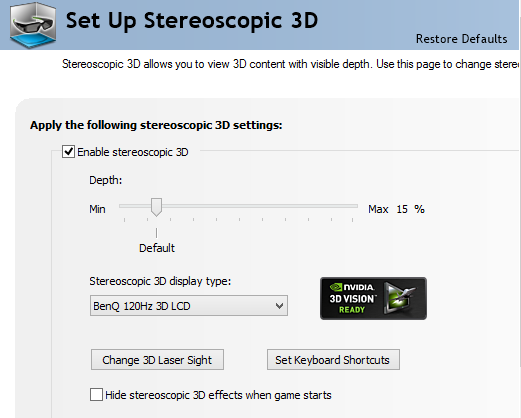
Note the "Stereoscopic 3D display type" box. You should set it to your monitor, and then press Apply. If instead it is set to "3D Vision Discover", the video driver will assume that you are using colored glasses instead of LCD shutter glasses, and show a different type of stereoscopic image that does not work with the NVidia 3D Vision glasses.

Startup

To use MuJoCo HAPTIX as a generic simulator and bypass all motion-capture initialization, run it with the single command-line argument "-nomocap" as follows:

mjhaptix -nomocap

Note that you can specify a command-line argument when running the program from a desktop shortcut: right-click the shortcut, select Properties, then select the Shortcut tab and enter the command-line argument after the program name in the Target field.

Running MuJoCo HAPTIX without "-nomocap" shows a welcome screen and displays progress of the OptiTrack initialization - which either succeeds, or fails with an error message. Possible reasons for failure are:

The OptiTrack is disconnected or powered down,
Motive or another instance of MuJoCo HAPTIX is already running,
The file "project.ttp" was not found in the program directory, or is corrupted,
The expected names and number of rigid bodies and/or markers were not found in "project.ttp",
NPTrackingToolsx64.dll or libiomp5md.dll was not found.

The latter two DLLs are the OptiTrack library and Intel's OpenMP library which the OptiTrack software uses. MuJoCo HAPTIX looks for them under their default installation directory (Program Files\OptiTrack\Motive) as well as in the system path. If Motive was installed at its default location these DLLs will be found automatically. If for whatever reason they are not found, locate them manually and copy them to the MuJoCo HAPTIX program directory. libiomp5md.dll has 32-bit and 64-bit versions. We need the 64-bit version.

If any of the above error conditions are encountered, the program shows an error message and continues with the motion capture-related Toolbar items disabled (same as if it was started with "-nomocap"). In this mode it can still be used over the API as well as with the interactive mouse controls and SpaceNavigator. This is useful if you want to work on a second computer that does not have an OptiTrack connected to it. Do not install Motive on this second computer; it will not run without OptiTrack hardware.

MuJoCo HAPTIX has a socket API which requires opening a socket for listening and accepting connections from user programs. The first time you run the software, Windows will automatically show the following dialog:

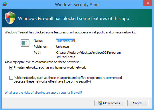
Click "Allow access". This will create an Inbound rule in the Windows Firewall the program to listen for incoming connections. If you click Cancel, it will create a rule blocking connections - in which case you can still connect to it from the local machine but not from a remote machine.

The software has a built-in mechanism for update notifications. On startup it connects to www.mujoco.org, parses the webpage listing the available versions, and prints a message in the lower-right corner indicating if a new version is available or if the software is up to date. This mechanism will not work if your computer is not connected to the Internet or you have firewall policies in place that prevent the software from accessing the Internet. Updating is done manually. The automated mechanism described here only shows notifications, and is designed to remain as unobtrusive as possible; the notification disappears as soon as you load a model.

Auxiliary files

Every time MuJoCo HAPTIX exits in a normal way, it updates the file "defaults.mjs" in the same directory as the executable. This is a binary file in custom format. It keeps the data from the Settings / Sim dialog as well as the list of recent files from the file menu. If this file is deleted, the settings will revert to their defaults and the recent file list will be cleared.

When errors or warnings are internally generated, the software creates the file "MUJOCO_LOG.TXT" if it does not already exist, in the same directory as the executable. It then writes the error/warning message in this file, preceded by the date and time. New messages are appended at the end of the file. Two common types of messages are warnings that the simulation went unstable (which happens when experimenting with physics parameters or performing extreme actions), and that a socket error was detected - usually because the user-side program quit while data was being exchanged. This log file is not needed for the operation of the software, and can be deleted.

Motive

Installation

The Motive software from NaturalPoint comes with the OptiTrack system. It is only needed when the motion capture features of MuJoCo HAPTIX are used. Motive is installed on the computers shipped to the HAPTIX teams, and can also be downloaded from the NaturalPoint OptiTrack downloads website. We need the 64-bit version. The installer asks for permission to install a number of prerequisites; all of them are needed.

Motive can stream real-time data, similar to software that comes with other motion capture systems such as Vicon and PhaseSpace. This however is NOT how we use it. Instead, MuJoCo HAPTIX loads the OptiTrack library (NPTrackingToolsx64.dll) at runtime. This library provides similar functionality as Motive but without the GUI and graphics. The only use of Motive is to adjust the camera view and create/edit the project file "project.ttp" as explained below. This project file is then loaded by MuJoCo HAPTIX at runtime.

Motive/TrackingTools has a built-in license which is activated when OptiTrack V120 hardware is discovered (this is the license we use). It can also be used without motion capture hardware, or with higher-end hardware, by purchasing a separate license. As a result, if you start Motive when the OptiTrack is disconnected or powered down, it will issue an error about missing license rather than missing hardware. License-related errors also occur if you attempt to start both Motive and MuJoCo HAPTIX, or two instances of either software. This is because the first instance takes possession of the OptiTrack, and the second instance cannot find an OptiTrack to activate its built-in license.

Configuration

The Motive software is used to adjust the cameras and create/edit the project file "project.ttp" in the MuJoCo program directory. The goal is to achieve this general configuration:

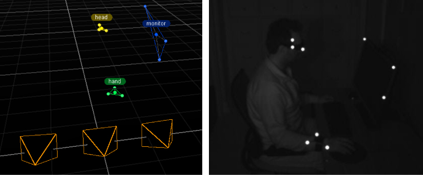
These are screenshots from Motive in our setup. The right image is the 2D view from one of the cameras. By default Motive only shows markers, but you can also enable greyscale images from the context menu (Right-click over the image). Note that it is better to interact with the MuJoCo HAPTIX VE while standing, with the monitor elevated as far as the stand will go. The sitting position in the above images is merely for taking sreenshots.

The left image is the perspective 3D view (again enabled from the context menu). The markers belonging to each body are grouped and the bodies are named accordingly. MuJoCo looks for the body names in the project file, so they must be "monitor", "head", "hand". The order is not important. Each body must have exactly 3 markers assigned to it.

The MuJoCo HAPTIX distribution has our "project.ttp" file in the program directory, but you have to edit it because your marker configuration may be slightly different. The Motive user interface is reasonably straightforward. Briefly, select the body you want to modify and delete it. Then select the 3 markers that just became unassigned (by dragging a rectangle around them), go to Menu/Layout/Create, this will open a panel on the right - where you press Create from Selection. The body is now created but it has a generic name. Click on the newly created body in the 3D view to select it, and change its name in the panel on the right.

One more setting we need to adjust is the intensity of the infrared LEDs built into the cameras. The OptiTrack documentation recommends leaving them at maximum but this only makes sense for large capture volumes. Here we need to lower the intensity, for the following reason:

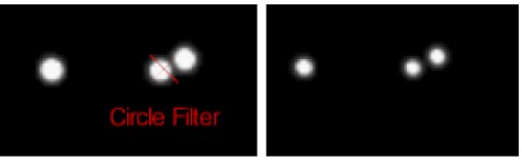
Apart from occasional marker occlusions, the biggest challenge in terms of motion capture is two markers getting too close in the camera view. Since the cameras are relatively close to each other, if two markers overlap in one view they will overlap in all views, causing the corresponding rigid body to be lost. In fact the more markers we attach to a given body, the worse this problem becomes - so the optimal number of markers per body appears to be 3, somewhat surprisingly. When two markers overlap completely there is nothing to be done (other than moving the hand to a different pose). But the more common scenario is that markers come close without overlapping. With the default settings this is sufficient to break the tracking algorithm. See left panel above. The problem is that the high LED intensity causes "blooming" of the markers. Reducing the intensity from 15 to 5 yields the image on the right, where the markers appear smaller and the problem is resolved. An added benefit of reduced intensity is that it can eliminate reflections from nearby shiny objects and surfaces. How far you can reduce the intensity depends on your setup.

Once the bodies are re-created with your marker configuration and the LED intensity is adjusted, save "project.ttp" in the MuJoCo HAPTIX program directory.

Apart from creating the project file, Motive is helpful in terms of positioning and orienting the cameras. Our suggested layout was shown above, but you should experiment and find out what works for you. Maximize the 3D perspective view in Motive (so you can see it from a distance), put on the glasses and hand-tracking tool, elevate the monitor as it would be during a session, and make the movements you expect your subjects to be making. If the OptiTrack loses one of the bodies, the corresponding image will freeze until the body is found again. Thus your goal here is to arrange the setup so that none of the bodies are freezing. The hand body is the one that is potentially problematic, especially during rotations. Moving the cameras closer helps, but you cannot move them too close because the head and monitor also need to remain in view. Keep in mind that your subjects may be taller than you - so there should be some room in the vertical direction.

MuJoCo HAPTIX does not rely on the cameras remaining in place. It tracks the head and the hand relative to the monitor (which is why we have markers on the monitor), so you can move the cameras around after the project file is saved. In fact you can even move them during an experimental session.

Compatibility

MuJoCo HAPTIX uses certain functions provided by NPTrackingToolsx64.dll which comes with Motive. This DLL in turn relies on libiomp5md.dll which is Intel's OpenMP library. If these DLLs are updated to newer versions, they may become incompatible with MuJoCo HAPTIX. Intel's OpenMP library is stable, however Motive is being actively developed, which can cause compatibility issues. Here is a table showing compability among recent versions of Motive and MuJoCo HAPTIX:

HAPTIX
0.98 - 1.10 HAPTIX
1.20 - 1.50

Motive 1.7.2 YES YES

Motive 1.8.0 NO YES

We will keep this table updated for future releases of MuJoCo HAPTIX. In addition, as of MuJoCo HAPTIX 1.20, the user can update their Motive installation (for other projects) and continue to use an earlier Motive version with MuJoCo. This is done by simply copying NPTrackingToolsx64.dll and libiomp5md.dll from the older Motive version in the MuJoCo HAPTIX program directory. The DLL loader checks the executable directory before the standard Motive installation directories, which are:

\Program Files\OptiTrack\Motive\lib\NPTrackingToolsx64.dll
\Program Files\OptiTrack\Motive\libiomp5md.dll

Note however that if Motive changes its project file format (for .ttp files), newer project files will not work with MuJoCo versions that do not support them, even if the DLLs are copied as explained above.

User interface

Toolbar

The GUI in MuJoCo HAPTIX is centered around the toolbar, which has the following appearance:

The available tools can open and close other GUI elements, or apply commands to the simulation. Some tools can be toggled (e.g. the Pin tool in the above image), while others can only be clicked and do not have an underlying state. Hovering with the mouse over a tool shows a tooltip, including the tool name/function and its keyboard shortcut if available. At startup most tools are disabled because they require a model. Once a model is loaded they become active.

The function of the tools is as follows:

Tool Key Desciprtion

Pin Toolbar. When this tool is toggled, the toolbar is always visible. When this tool is not toggled, the toolbar is visible only when the mouse is over it, and hidden otherwise. Use this tool to hide the toolbar if it becomes a distraction - for example in full screen mode where you may prefer to focus on the rendering.

File Menu. This is a traditional file menu. We have opted against a menu bar because it makes little sense in full screen mode. At the top of the file menu there is a list of recently opened models (in blue). Open can be used to open models in XML and binary format. Save can used to save models in XML and binary format, as well as a plain text format which is a human-readable model description. Print Data can be used to print the entire workspace into the file MJDATA.TXT for model debugging.

F1 Help. Open and close the Help dialog. Note that all dialog windows can be closed from their close button or from the toolbar, and re-opened again later at any time. The Help dialog has four tabs: Interaction, Commands, XML, About.

F2 Settings. Open and close the Settings dialog. This dialog contains all user-adjustable settings. It has three tabs: Sim, Physics, Render. Note that the Settings dialog (as well as the Sliders dialog) can be docked on the left or the right edge of the main window, and the tabs in it can be rearranged using the mouse.

F3 Sliders. Open and close the Sliders dialog. This dialog is used to manually adjust joint angles and control signals. It has two tabs: Joint and Control.

F4 Info. Open and close the Info box in the lower-left corner of the main window. Unlike the above dialogs which are regular GUI elements, this is passive text generated as part of the OpenGL rendering, and updated at the same rate as the 3D graphics. It conveys information about the state of the simulation.

Ctrl+N Sensors. Open and close the Sensor data box in the lower-right corner of the main window. This is a bar graph showing normalized sensor data in real time.

Ctrl+F Profiler. Open and close the Profiler box on the right of the main window. This is an elaborate plot showing information about the internal operation of the physics simulator. It can be used to fine-tune complex models.

F5 Full Screen. Switch between windowed mode and full screen mode. You can also maximize the window with the usual controls, but that will leave the title bar and task bar visible - which you probably want to avoid when working in full screen mode.

F6 Stereo. Switch between stereoscopic and regular rendering. The software starts in regular mode. If the video card supports quad-buffer OpenGL and the monitor is set to 100Hz or higher, the software generates frame-sequential stereo. Otherwise it generates side-by-side stereo.

F7 Head Camera. When enabled, the camera tracks the head of the user (or rather, the NVidia 3D Vision glasses with markers attached to them). Use head tracking together with full screen mode and stereoscopic rendering.

F8 Motion Capture. When enabled, the position and orientation of the first mocap body defined in the model tracks the data arriving from the OptiTrack. This mocap body is usually connected to the floating base of a robot model via a weld equality constraint, allowing the user to move the entire robot.

F9 Record Log. Start and stop recording. A new log file is created in the datalog directory every time recording starts.

Space Run / Pause. Switch between simulation mode and paused mode. The current mode is indicated by the state of this tool, but since it is essential for the user to be aware of the mode the software is in, we also print "Paused" in large font in the lower-right corner when in paused mode.

Back
Space Reset. Reset the simulation state to the reference configuration defined in the model. When instability is detected, the simulation resets automatically. Use this button whenever things go wrong. If the simulation is repeatedly going unstable as soon as you reset, this means your physics settings are causing unstable numerical integration.

Ctrl+L Re-Load. Re-load the last successfully loaded model (i.e. the model you are currently simulating). This is useful when you are making changes to the XML. It differs from Reset in that all model settings (including the physics options) are restored, and not just the simulation state.

Ctrl+A Re-Align. Center the camera view at the geometric center of the model - which is computed at compilation time, and is not necessarily accurate after the bodies start moving. This command only works with the Free camera. It is useful if you manipulate the camera in an undesired way, or otherwise lose the relevant parts of the model.

Loading models

MuJoCo HAPTIX (as well as MuJoCo Pro) can load models in its native XML format called MJCF, its native compiled binary format called MJB, and the URDF format. Model files can be loaded in several ways:

From the standard Open dialog in the File menu. Navigate to the model directory and select the desired file;

From the list of recent files in the File menu; simply click on the model you want to load. This is often the easiest way to load previously used models;

Dragging a model file and dropping it over the main application window. The software will not allow you to drop files with invalid extensions; only .xml, .urdf and .mjb are allowed.

Regardless of which method is used to specify a model file, if the file is XML, it will be parsed and then compiled. If both operations are successful the model will appear in the 3D window and will be ready for simulation. In case of parse or compile errors, the first error will be printed in a message box and the simulator will continue to use the last successfully loaded model. When loading a compiled binary file (MJB), it is usually impossible to obtain an error because this model has already been used. The only exception occurs when loading an old MJB file which is no longer compatible with the software; this will trigger an error message.

Saving models

The Save menu becomes active only after a model is loaded. The model can be saved as MJCF, MJB or plain text. The latter format provides information to a human reader but cannot be loaded back in the software. Saving to MJCF uses a subset of the MJCF format as described in the Modeling chapter.

There are several reasons to save a model:

Saving as MJB produces a single binary file with all assets (meshes and textures) baked in. This model file does not have any dependencies and can be moved to a different directory/computer. It also loads faster, because it is essentially a memory dump of the runtime model representation. However the XML parser and compiler are also very efficient, so the difference in load time is only noticeable for models that have large meshes or textures;

If the user adjusts the physics settings of the model, it may be desirable to save the model. The new settings will be saved. Note however that the state of the simulation is not saved; instead the state is initialized to the reference configuration at load time and also during reset;

The GUI can be used to create keyframes, corresponding to special model configurations that are of interest to the user. When saving the model, these keyframes will be saved (in both the MJCF and MJB formats). The model can be reset to a selected keyframe from the Settings / Sim dialog. Note that the number of keyframes is specified in the model definition and cannot be changed from the GUI; only the content of the predefined keyframes can be changed.

Recording and playback

MuJoCo HAPTIX has data recording and playback capabilities. The Record button on the toolbar starts data recording. This creates a new file in the datalog directory. The file names are generated automatically and are in the format modelname_N.mjl where the modelname is taken from the model (not necessarily the same as the filename) and N are increasing integers. Note that this is a change introduced in MuJoCo HAPTIX 1.40; previously there were only 50 slots available for log files, now they are unlimited.

The recording ends when the Record button is pressed again (so that it becomes un-toggled) or when a model is loaded or re-loaded. During recording, the sign "recording" is shown in the lower-right corner of the screen. If this sign is not shown, the software is not recording data. The data is streamed to disk continuously, so if the software crashes unexpectedly the data should not be lost.

The log file is a binary file with custom format. It contains everything needed to fully reconstruct the simulation state: timestamp, positions, velocities, controls, mocap body positions and orientations, and sensor data. This combines the information from the data structures mjState, mjMocap, mjControl, mjSensor described below. All this information is saved at each simulation time step by default. In some cases this may generate too much data. MuJoCo HAPTIX allows the recoding to be sub-sampled, using the "Skip timesteps" field in the Sim dialog described below. When this setting is 0, data is saved at every time step. Values greater than 0 specify the number of time steps to be skipped when saving.

The log files can be opened, analyzed and played back using MATLAB. The function readlog.m in the apimex directory opens the log file, and returns a data structure with all the information in it. To play back the simulation, call playlog.m with the data structure provided by readlog.m as argument. This opens a MATLAB figure with playback controls, and a plot of the timestamp over frames. If the simulation was reset during recording, this plot goes to zero, indicating trial boundaries. This function expects MuJoCo HAPTIX to be started, and paused so that the playback does not fight with the simulator. The same model as used for data recording must be loaded; only the model name can be different. The playback mechanism uses the socket API described below to send the simulation state from MATLAB to MuJoCo HAPTIX, which then renders it.

The log file contains a description section followed by a data section. The description section contains the following information:

  nq:           length of position vector qpos
  nv:           length of velocity vector qvel (also equal to number of degrees of freedom)
  nu:           length of control vector ctrl
  nmocap:       number of mocap bodies
  nsensordata:  number of scalar sensor readings
  name:         model name

Each variable in the data section is a matrix, with rows corresponding to the different MuJoCo fields, and columns corresponding to the time step when data was saved. Thus all matrices have the same number of columns. When the variable corresponds to a 2D MuJoCo array, it is serialized into the rows of the corresponding matrix. The data section contains the following information:

  time:         simulation time
  qpos:         position vector
  qvel:         velocity vector
  ctrl:         control vector
  mocap_pos:    mocap body positions, with size 3*nmocap
  mocap_quat:   mocap body quaternion orientations, with size 4*nmocap
  sensordata:   sensor data array

As of MuJoCo HAPTIX 1.40, we have added a stand-alone command-line utility to play log files. This does not require MATLAB or MuJoCo HAPTIX; it contains its own copy of MuJoCo statically linked. The executable is playlog.exe in the program directory. Open a command prompt, cd to the program directory, and start playlog with two command-line arguments: the model filename, and the log filename. For example:

  playlog ..\model\MPL\MPL_Basic.xml ..\datalog\MuJoCoModel_1.mjl

Note that the log filename contains "MuJoCoModel" rather than "MPL_Basic" because the XML model MPL_Basic.xml does not define a model name, and so MuJoCo uses the default model name which is "MuJoCo Model". Spaces are omitted from the log filename. One can provide an optional third argument which is the GUI font scale; it can be 100, 150 or 200.

The above command opens a window which looks like this:

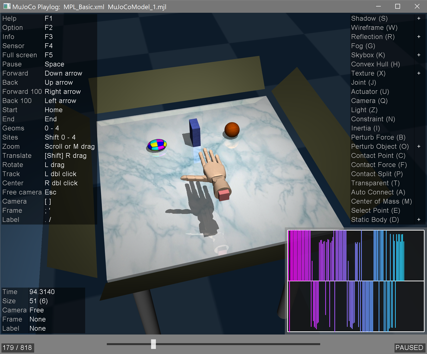
The help on the top-left lists all available commands. The menu on the top-right correspond to all visualization options; only keyboard shortcuts can be used to toggle these options, not the mouse. The info text on the lower-left shows the simulation time, number of active scalar constraints and contacts, as well as the camera, frame and labeling modes (which can be changed via keyboard shortcuts listed in the help panel). The plot on the bottom-right shows the sensor data recoded in the log file. Each sensor corresponds to one vertical bar. In this model we have too many sensors defined, but most models have fewer sensors so the plot is more readable. Each sensor is normalized over the entire recording duration. All four panels can be hidden by pressing F1 - F4 respectively.

The bar on the bottom shows a slider that can be moved with the mouse as well as keyboard shortcuts show in the help panel. When the playback is running, the slider advances automatically. The text to the left of the slider shows the current data frame and the total number of data frames in the log file.

Note that mouse perturbations cannot be used here because the motion is pre-recorded, however the camera can still be controlled with the mouse, in the same way as in MuJoCo HAPTIX. In this way the animation can be viewed from different angles.

Help dialog

The help dialog is always available, even before a model is loaded. The About tab shows the software version and list of open-source libraries used, and points the reader to the license file in the program directory. The XML tab shows a table with the XML elements and corresponding attributes that are allowed in the MJCF format. This is a convenient reference when editing models in a text editor, but the full documentation in the Modeling chapter is usually needed as well, at least while learning MJCF. The Interaction and Commands tabs summarize the mouse and SpaceNav interaction as well as the toolbar and keyboard shortcuts.

Settings dialog

This dialog is used to adjust all settings in the software. It becomes activate only after a model is loaded. It can be closed at any time from the toolbar or the close button on the dialog window, and can be opened again later from the toolbar (or using the keyboard shortcut F2). By default only one tab is shown at a time, however the tabs can be rearranged with the mouse so as to expose more than one. Below we show all three tabs exposed:

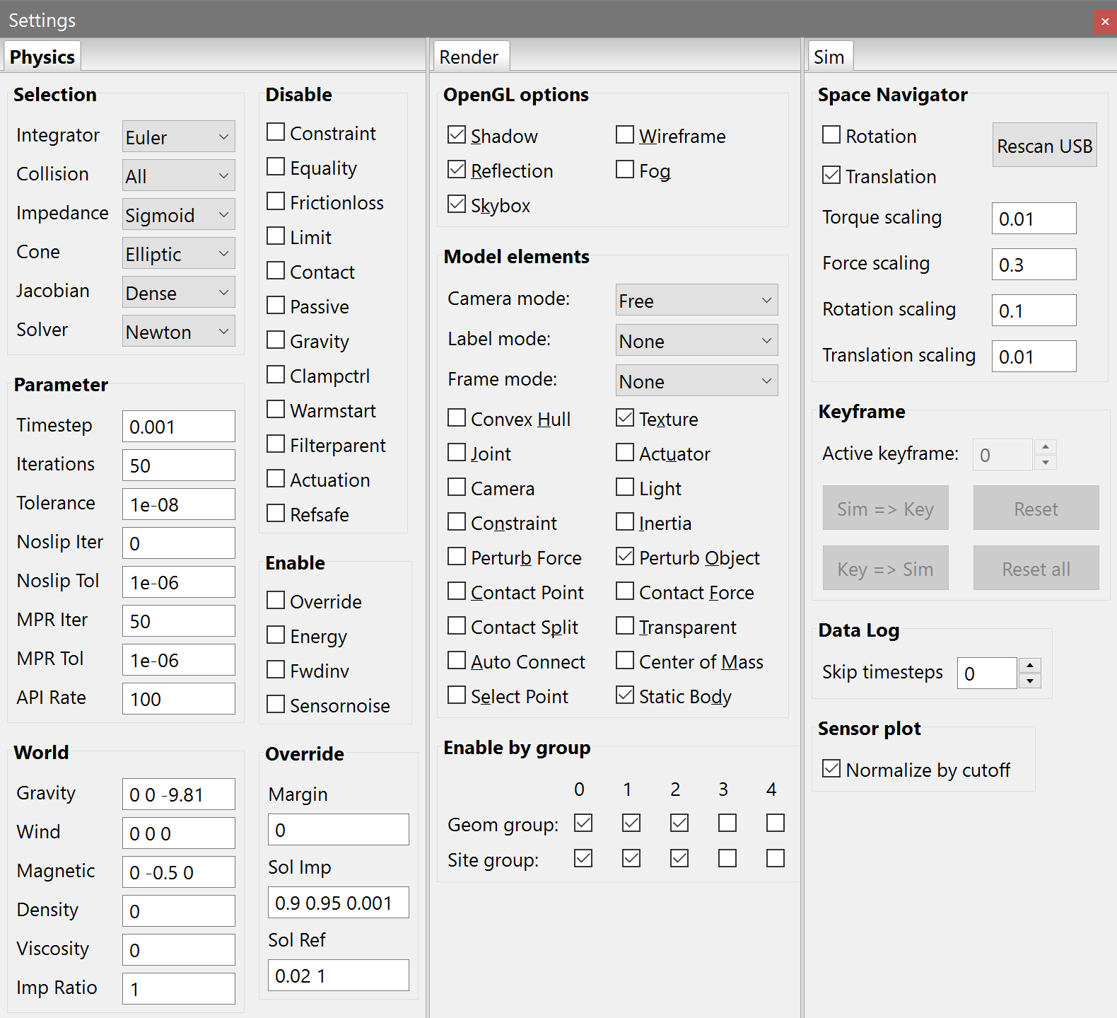
Physics tab

This tab is in one-to-one correspondence with the mjOption structure which is part of mjModel. See the option documentation in the Modeling chapter. These settings can in principle be modified at each timestep, although in practice they are usually modified while experimenting with the model and adjusting its properties, and fixed afterwards.

Render tab

This tab controls the 3D rendering. The settings here enable and disable various rendering features. The actual appearance of the objects is defined in the model. All check boxes in this dialog have keyboard shortcuts, as documented later and also shown in brackets here. They can also be revealed by pressing the Alt key when the tab is active (as in the above image). The reason for introducing all these shortcuts is because it is convenient to change the visualization settings during a simulation, so as to emphasize the model elements and physics effects that are currently of interest.

Shadow (S): Shadow rendering. Each shadow-casting light defined in the model is processed in a separate OpenGL rendering pass, using rendering to texture to simulate shadow effects. This requires OpenGL 3.2 or later; if the video card or driver do not support OpenGL 3.2, no shadows will be rendered.
Wireframe (W): Render all objects using lines instead of polygons. The line width is part of the model definition. This mode is useful for examining the details of the meshes.
Reflection (R): Reflection rendering. Reflections are currently only rendered on planes, even though the material definitions in the model allow reflection coefficients for all objects. This is done using the stencil buffer; therefore if the implementation does not support stencil buffers the reflections will not be visible. Each reflecting plane adds an OpenGL rendering pass.
Fog (G): Enable fog rendering. This makes distant objects dark. The distances from the camera at which fog starts and ends are defined in the model.
Skybox (K): Enables rendering of a "skybox" which is a textured box far away from the camera. This is normally used to create a distant background. Note that the box is automatically centered at the camera, so it will appear to be stationary in eye coordinates - much like a mountain in the distance appears to be stationary in eye coordiantes. The first texture defined in the asset section is used to render the skybox. This would normally be a cube texture, with 6 different PNG files for the different sides of the cube. If no textures are loaded, this setting has no effect.
Camera mode: This selection box can be used to select the OpenGL camera. When the head-tracking camera is enabled, it overrides this setting. The list of available cameras includes the default Free camera (which can be manipulated with the mouse) as well as any fixed cameras defined in the model. The latter can be attached to moving bodies and provide dynamic views.
Label mode: Automatically generate text labels for all objects of the type selected in this box. In addition to the standard model element types, one can choose Selection which labels the selected body, and Select Point which labels the point used to select the body. Only elements that are currently rendered (as specified by the check boxes) are labeled. The default setting is None which removes all labels. The labels are rendered over the 3D graphics and ignore the z-buffer, meaning that you can see labels for occluded objects as well. We have taken steps to enhance the text contrast when rendering on light background. Still, when two labels are on top of each other there is no way to see the one at the back. The order depends on the ordering of the model elements.
Frame mode: Render a right-handed coordinate frame for all objects of the type selected in this box. The axis convention is x:red, y:green, z:blue.
Convex Hull (H): Render the convex hulls of the meshes instead of the actual meshes. This only has an effect if the mesh is non-convex to start with, and its convex hull has been computed at compile time - which happens if the mesh is enabled for collisions.
Texture (X): Render textures. When disabled, textured geoms appear with uniform color taken from the material definition or the geom rgba field.
Joint (J): Render joints. Hinge joints are rendered as arrows without wedges. The arrow starts at the joint center. The right-hand rule can be used to infer the positive direction of motion. Slider joints are rendered as arrows with wedges. Ball joints are rendered as spheres. Free joints are rendered as cubes. To see the joint names, you must both render the joints and enable joint labeling.
Actuator (U): Render actuators. Only motors attached to hinge and slide joints are presently rendered. The right-hand rule can again be used to infer the positive direction of motion.
Camera (Q): Render the cameras defined in the model, using decorative elements. The free camera and the currently active camera are not rendered.
Light (Z): Render the lights defined in the model, using decorative elements. The headlight attached to the active camera is not rendered.
Constraint (N): Render constraints. These are cylinders connecting the points that are supposed to coincide.
Inertia (I): Render an equivalent inertia box around each body. This box is centered at the center of mass and is aligned with the principal axes of inertia. Its sizes are computed from the mass and inertia matrix of the body, under a uniform density assumption. Note that some poorly constructed models have large body inertias compared to body mass, resulting in very large equivalent inertia boxes.
Perturb Force (B): Render the applied/perturbing force as an arrow.
Perturb Object (O): While perturbing the selected body with the regular mouse, render the reference position and orientation of the spring-damper used to generate perturbing forces.
Contact Point (C): Render the contact points as cylinders. The cylinder axis points along the contact normal direction.
Contact Force (F): Render the contact force as an arrow.
Contact Split (P): Split the contact force into normal and tangential components, and render two arrows per contact.
Transparent (T): Increase the transparency (i.e. reduce the alpha value) of all geoms attached to moving bodies. This is done on top of any transparency defined in the model. This rendering mode can reveal geometric aspects of the model that are hard to see with opaque surfaces.
Auto Connect (A): Automatically generate a "skeleton" by connecting the joints and body centers of mass along the kinematic tree.
Center of Mass (M): Render a sphere corresponding to the center of mass of each kinematic tree.
Select Point (E): Render a sphere denoting the point that was clicked in order to select a body. This point is in the local coordinate frame and therefore moves with the body. Its coordinates can be printed with the Select Point choice in the Label mode box. This mode is useful if you need to find out the local or global coordinates of a given visual feature.
Static Body (D): Enable rendering of static bodies (such as the ground plane). When disabled, only dynamic objects are rendered. This is useful when you need to focus on the model and ignore the environment.
Geom group (0-4): Geoms are assigned to groups as defined in the model. These groups do not affect the simulation but are used to show and hide the geoms by group. If the group number of a geom is outside the range shown in the dialog (0-4), it is clamped to the nearest valid group number for rendering purposes. Note that some models have geoms in groups that are disabled by default. This is done to hide visual details that are only needed in special circumstances.
Site group (Shift 0-4): Same as geom groups, but applies to site groups instead. Sites in MuJoCo can be used for different purposes, including routing of tendons, specifying slider-cranks, touch sensors, IMUs, and locations of interest to the user. Sites are normally defined in the model with shape and appearance that groups them according to their intended use. The site group attribute can be used for further grouping, allowing all sites in the same group to be shown/hidden together.

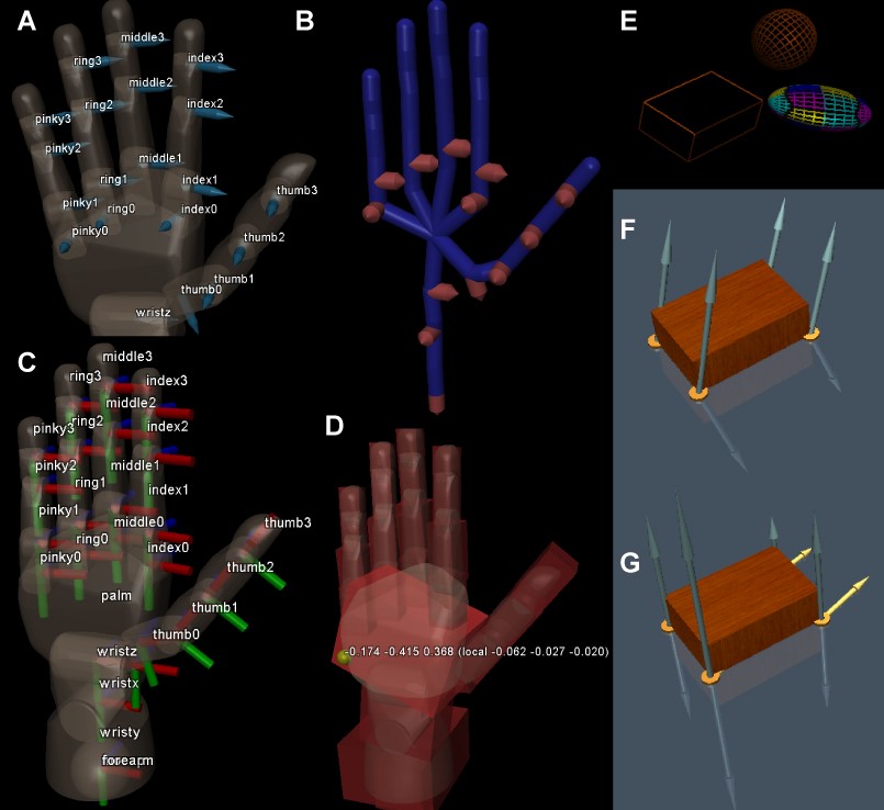
The above image illustrates several of the rendering features. Panel A shows transparency, joint arrows and joint labels. Panel B shows the auto-connect skeleton and actuator rendering. Panel C shows transparency, body frames and body labels. Panel D shows transparency and equivalent inertia boxes, along with the selection point and its local and global coordinates. Panel E shows wireframe rendering. Panel F shows reflections, textures, contact point and contact force rendering. Panel G shows the split of contact forces into normal and tangential components.

Sim tab

This tab contains application-wide settings that are related to the GUI. They are grouped as Simulation, SpaceNavigator, and Keyframe. Their meaning is as follows:

Rescan USB: When the software first starts it scans the USB ports for SpaceNavigator devices, and connects to the first one that is found. If however a SpaceNavigator is connected to the computer later, the software will not detect it automatically. Instead you need to press this button to trigger another scan of the USB ports.
Rotation and Translation: These check boxes enable/disable the rotational and translational components of the SpaceNavigator input. The reason to disable one or the other is because it if difficult for a human hand to control both 3D rotation and 3D translation accurately at the same time. Note that the state of these check boxes can also be toggled using the two buttons on the device: the left SpaceNavigator button enables/disables rotation, the right button enables/disables translation.
Torque and Force scaling: The SpaceNavigator data is in some arbitrary units, which have to be mapped to forces and torques applied during perturbations. These edit boxes define the scaling from device units to physical units. Adjusting these parameters alters the SpaceNavigator sensitivity, i.e. a larger Torque scaling value will apply greater torque to the selected object for the same rotation of the SpaceNavigator. The actual force/torque being applied also scales with the average mass of the bodies in the model. The latter scaling reduces the need to change these settings for models with different mass and dimensions, but still, occasional adjustment is needed.
Rotation and Translation scaling: These settings are similar to the above, except they are applicable when the SpaceNavigator is used to directly move and rotate a body (kinematically), as opposed to exerting forces and torque on the body. See body perturbations for details.
Active keyframe: The number of the keyframe you want to work with. When a model is loaded, the number of predefined keyframes (mjModel.nkey) is used to set the maximum value available in this selection box. If the model has no keyframes, this entire panel is disabled. Note that when you change the keyframe selection nothing happens; this box merely selects the keyframe for subsequent actions applied through the buttons described next.
Sim => Key and Key => Sim: These two buttons are used to copy the current state of the simulation into the selected keyframe, and to copy the state saved in the keyframe back in the simulation. The state includes the positions and velocities of all degrees of freedom, the activations of any actuators that have internal dynamics, and the simulation time. All these quantities are saved when the model is saved.
Reset and Reset all: The Reset button is used to reset the selected frame. This means setting the time, velocity and actuator activations to 0, and the position to the model reference configuration (mjModel.qpos0). The Reset all button does the same for all keyframes and not just the selected one. Use this button with caution; there is no warning before resetting all keyframes.
Skip timesteps: Specifies the number of time steps to skip (or sub-sample) during recording. If this value is 0, data is recoded on every time step (assuming the Record button is pressed). If this value is 4, data is recorded on every 5th time step.
Normalize by cutoff: When this box is checked, the sensor data plot is normalized by the cutoff value for each sensor (if defined in the model). When the box is unchecked, the raw sensor data are plotted.

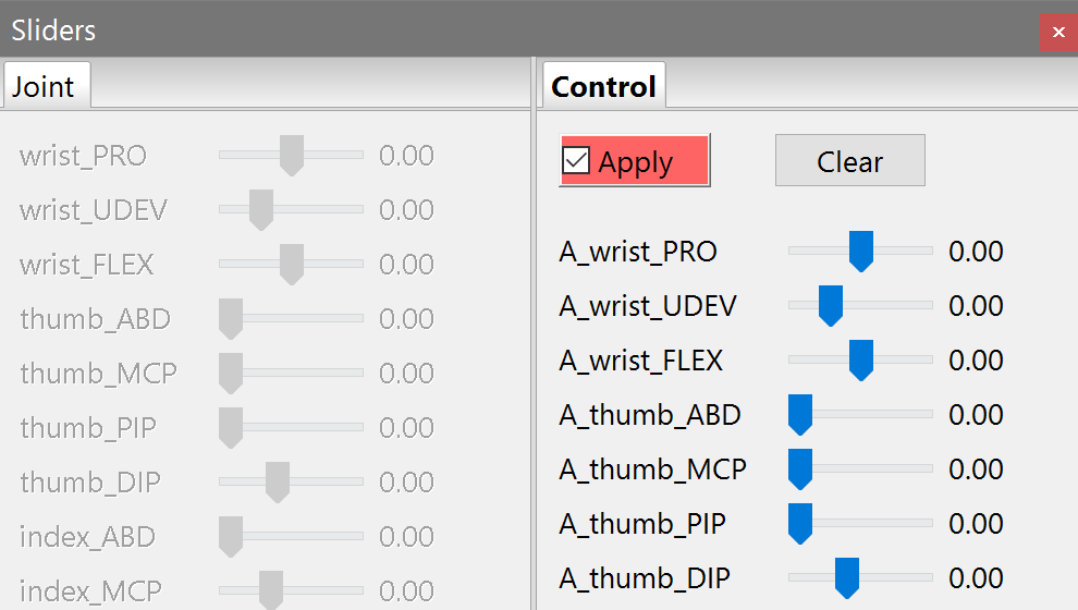
Sliders dialog

This dialog for used for manual adjustment of joint angles and control signals. It is automatically re-populated every time a model is loaded. It can be docked along the left and right edges of the main window. It has the following appearance (only the top portion is shown):

Joint tab

This tab shows the list of scalar joints in the model (i.e. hinges and slides). If joint limits are defined in the model, they are used to set the range of the corresponding slider. Otherwise the range is set to default values: +/- pi for hinges; +/- model extent for slides. This tab is only activated in paused mode; in sim mode it is disabled and the sliders do not track the animation. Sometimes the joint position shown on the right of the slider may appear in red. This means that the actual joint position is outside the range of the slider - and therefore it will "jump" as soon as you touch the slider. This out-of-range phenomenon can occur when you simulate and then pause. Since the constraint model is soft, joint limits can have some violation during simulation.

Note that floating bodies are "connected" to the world with a free joint which does not appear in this dialog. To move floating bodies in paused mode, use the mouse or SpaceNavigator.

Control tab

This tab shows the list of actuators in the model. The sliders can be used to set the control signals for the actuators. The slider range is as specified in the model, or +/- 0.1 if the specification is missing. Recall that each actuator in MuJoCo has a scalar input (the control signal) and a scalar output (the actuator force) which is mapped to joint torques; servos and other actuators that have built-in control circuitry requiring multiple inputs are modeled via user code. Thus the visible effects of the Control sliders depend on the type of actuator: for a position actuator whose control input is reference position, the slider will effectively control the joint angle; for a motor actuator whose control input is torque, the slider will generate constant torque which may push the joint to its limit.

This tab is only active in simulation mode (the opposite of the Joint tab). Unlike the Joint tab where the sliders have immediate effect on the model configuration, the Control tab only has an effect when the Apply box is checked. This is because the actuator controls would normally be specified from user code over the socket API. The Control tab makes it possible to override those controls and experiment with the model manually. When the simulation is reset or a new model is loaded, the Apply box is automatically unchecked.

Info box

This GUI element is not a window, but rather a see-through text overlay generated by the OpenGL rendering in the lower-left corner. It can be enabled and disabled only from the Info tool in the toolbar, and cannot be moved or resized. Which items appear in this overlay depends on the state of the simulation. The possible items are:

Remote: Shows the status of the socket connection to a user program. The possible values are "Waitning" and "Connected". When MuJoCo HAPTIX starts it opens a TCP/IP socket for listening, and accepts the first connection request. If this connection breaks or is closed upon request from the user program, it goes back to listening mode.
SpcNav: Shows the status of the SpaceNavigator connection. The possible values are "Found" and "Not found". Note that you can rescan the USB ports for newly-connected devices from the Settings / Sim dialog.
Time: The simulation time in seconds; same as the time stamp provided over the socket API. This time resets to 0 when the simulation resets or when a new model is loaded, and pauses in paused mode. It is advanced by the numerical integrator (and not the CPU clock). The value in brackets is the realtime factor, computed internally by comparing elapsed simulation time to elapsed CPU time. The statistics are reset when the simulation resets. The realtime factor will normally track the target value specified in the Settings / Sim dialog.
CPU: CPU time per simulation step, in milliseconds. This is the key indicator of simulator efficiency. It tells you how far you can reduce the simulation timestep and still run in realtime. It is instructive to watch how the CPU time varies between models and contact configurations; having an intuition for these variations will tell you how far you can push MuJoCo when constructing new models or adding constraints to an existing model. In general, multi-joint dynamics are very fast to simulate (around 0.1 msec for a humanoid) while constraints (including contacts) can make the CPU time increase rapidly. The dense solvers have O(N^3) scaling with the number of active constraints. The sparse solver is O(N), but the constants are larger.
Size: Size of the constraint force vector being computed by the iterative solver. This size is strongly correlated with CPU time. The number of active contacts is shown in brackets. The constraint force vector includes joint and tendon limits, dry friction forces in joints and tendons, equality constraints, as well as contact forces (whose dimensionality can be between 1 and 6 depending on the model definition). When you disable constraints of a certain type in the Settings / Physics dialog, the size will decrease, assuming of course your model has constraints of that type.
FPS: Frames per second for the OpenGL rendering. The rendering is synchronized with the "vertical refresh" - which is better defined for CRT monitors than present-day LCD monitors, but is still present in video cards and drivers. You can override this synchronization from the NVidia control panel, by setting vsync to be off at all times. Then the FPS will normally increase up to 200 (we are limiting it internally); however this will not improve the effective rendering speed (because your monitor cannot respond this fast), and will interfere with stereoscopic rendering.
Energy: The sum of kinetic and potential energy, in Joules. The potential energy computation takes into account gravity as well as any passive springs defined in the model (but not the springs implemented by position actuators). When simulating energy-conserving systems, this measurement is very useful for assessing the overall accuracy of numerical integration; for such systems you should use the RK4 integrator. However when friction and unilateral constraints are present, the system does not have any conserved quantity. In that case the energy measurement can still be useful as an indicator of simulation stability; it should decrease in the absence of applied/control forces.
SolStat: Statistics about constraint solver convergence. The first number is the log10 of the residual gradient norm at termination. Smaller values mean more accurate results. Note that the tolerance option specifies the threshold value below which the solver terminates. The second number (in brackets) is the number of solver iterations applied at the current time step.
FwdInv: When the fwdinv option in the model is enabled, this field shows a different diagnostic of solver convergence: a comparison of the forward and inverse dynamics, in joint and constraint space. The results are shown in log10 units; smaller numbers indicate better convergence.
Mocap: When motion capture is enabled and the hand-tracking body is in view of the cameras, this field shows the number of milliseconds that motion capture data spends in the entire MuJoCo HAPTIX processing pipeline: from the time the OptiTrack driver delivered the data to MuJoCo, to the time the video driver reported that the corresponding pixels have been sent to the monitor. All additional latencies are due to the motion capture hardware/driver and processing inside the monitor.

Sensor data box

This is a bar graph showing the simulated sensor data. Each bar corresponds to one scalar reading. Sensors are automatically grouped by type, so that consecutive sensors of the same type are shown with the same color. If the box "Normalize by cutoff" in the Sim dialog is checked, the output of each sensor is normalized by its cutoff parameter, assuming the cutoff is positive. Otherwise the raw sensor data are included in the plot.

Profiler box

This is an elaborate plot with 4 subplots showing timing and other diagnostics about the operation of the physics engine. It can be used to fine-tune complex models; see MuJoCo Pro documentation. The profiler is the same as in the simulate.cpp code sample available with MuJoCo Pro.

Camera control

The "Camera mode" selection box in the Settings / Render dialog is used to select the camera for OpenGL rendering. There are a total of four camera types and subtypes in MuJoCo:

Head-tracking camera;
Free camera;
Free camera in object-tracking mode;
Cameras defined in the model.

Cameras defined in the model move with the body they are attached to, or remain stationary if attached to the world body. They cannot be manipulated interactively. The two varieties of the Free camera are of interest here with regard to interactive camera control via the regular mouse (not the SpaceNavigator).

The MuJoCo camera abstraction involves a high-level description (mjvCamera) and a low-level description (mjvCameraPose). The latter is used for actual rendering, and in the case of head-mounted cameras and model-defined cameras is controlled directly (by motion capture data or the simulator itself) ignoring the high-level description. In contrast, the free cameras are specified on the high level and the corresponding low-level description is computed internally at each video frame. This high-level description includes the following quantities:

fovy: Field-of-view in the vertical (y) direction. This value is specified in the model and cannot be changed interactively.
lookat: 3D global coordinates of the point where the camera is looking. The camera gaze direction corresponds to a ray and not a point, so this is just one point along the ray. Apart from defining the gaze direction, this point is the pivot point around which the camera rotates. The lookat point can be set via right doubleclick. It also moves when the camera is moved using right drag or shift + right drag.
azimuth: The azimuth angle of the camera (i.e. the rotation in the horizontal plane). This value can be changed interactively with left drag. Dragging in the horizontal direction changes the azimuth angle.
elevation: The elevation angle of the camera. This value can be changed interactively using left drag in the vertical direction. Note that the elevation angle is limited to the interval [-90, +90] deg, so the rotation will stop when you reach a camera pose looking directly up or down.
distance: Distance between the camera position and the lookat point (along the ray defined by the azimuth and elevation angles). This value can be changed interactively with scroll or center drag. It has the effect of bringing objects closer. The same visual effect can be achieved by moving the camera. The difference between the two becomes apparent when rotating the camera.
trackbody: When this feature is enabled via ctrl + right doubleclick, the camera starts tracking the body of interest. This is achieved by automatically moving the lookat point so that it remains fixed in the local body coordinates, modulo a low-pass filter making the camera motion smooth. The azimuth, elevation and distance can still be changed in this mode. Press Esc to exit tracking mode.

The relevant mouse and keyboard actions are as follows:

Action Description

Left Drag Change the azimuth angle. This results in rotation around the vertical (z) axis of the world.

Right Drag Move the lookat point in the vertical plane, defined by the z axis and the projection of the gaze axis in the horizontal plane. This results in moving the entire model up, down, left, right; up is defined relative to the world and not the monitor.

Shift +
Right Drag Move the lookat point in the horizontal plane. This results in shifting the model horizontally.

Left and
Right Drag Same effect as Shift + Right Drag.

Scroll Change the distance between the camera and the lookat point. This results in the model getting closer or farther away. It can be done with the scroll wheel of a mouse, or a scroll action on a trackpad.

Center Drag Dragging in the vertical direction has the same effect as Scroll. Dragging in the horizontal direction is ignored.

Right
DoubleClick Center the lookat point on the point that was clicked.

Ctrl + Right
DoubleClick Center the lookat point on the point that was clicked, and lock the lookat point in the local frame of the body to which the clicked point belongs. This results in tracking the body with the camera, through a low-pass filter.

Esc Stop tracking. The lookat point is set to its last position and remains constant until changed by another user action.

Note that holding the Alt key swaps the roles of the left and right mouse buttons, for both camera control and perturbations.

Body perturbations

Both the regular mouse and the SpaceNavigator can be used to apply perturbations to MuJoCo bodies. All perturbations are applied to the currently selected body - which is highlighted with a glow. Use left doubleclick to select a body (recall that the selection point and its coordinates can also be visualized by enabling the corresponding Render flag and labeling mode). Use left doubleclick over the background or over a static non-mocap body to clear the selection.

Once a body is selected, it can be perturbed in different ways depending on the type of body (Dynamic vs. Mocap), the device being used (Mouse vs. SpaceNav) and the software mode (Sim vs. Pause). The eight possible combinations are described in the table below.

Body Device Mode Description

Dynamic Mouse Sim To initiate perturbation, start dragging with the mouse while holding down the Ctrl key. The mouse commands are very similar to camera control: left drag rotates; shift + left drag rotates around a different set of axes; right drag translates in the vertical plane; shift + right drag (or left and right drag) translates in the horizontal plane. The rotations and translations are not applied to the body directly, but rather to the reference position/orientation of a spring-damper whose other end is attached to the selected body. The actual forces/torques are generated by this spring-damper; the stiffness and damping coefficients are defined in the model. To visualize this reference object, enable the Perturb Object flag in the Render dialog. The reference is set to the body position/orientation at the onset of the perturbation, regardless of where the mouse click occurs. Once you start dragging, the reference changes. When applying translations, only the position is changed and the perturbing object is rendered as an elastic band connecting the body and the reference position. When applying rotations, only the orientation is rendered - as a cube centered at the body. Note that if you rotate the reference orientation more than 180 deg away from the body, it will apply perturbing torque in the opposite direction. You can also visualize the perturbing force (but not torque) by enabling the Perturb Force flag in the Render dialog.

- - Pause In paused mode there is no spring-damper. Instead the perturbation is applied directly. However if the selected body is not a floating body, the perturbation will affect the root of the kinematic tree to which the selected body belongs - assuming this root is a floating body. If the root is not a floating body, the perturbation has no effect. This is because MuJoCo HAPTIX does not implement inverse kinematics. If you want to change the joint configuration, use the Sliders / Joint dialog. The mouse actions are the same as in simulation mode. No perturbation objects are rendered in this mode because there is no discrepancy between the body and the reference.

- SpaceNav Sim The SpaceNavigator is a 6D input device allowing simultaneous control over 3D force and 3D torque. However it is not always easy for a human to control both force and torque accurately, so we provide the option to enable one or the other or both. This is done from the check boxes in the Settings / Sim dialog. The two buttons on the physical device can also be used to toggle these check boxes. Only the translation component is enabled by default. The raw data generated by the device is scaled before applying it as a force/torque; see edit boxes in the Settings / Sim dialog. Similar to the mouse commands, the SpaceNavigator actions are aligned with the world rather than the screen; thus pulling the device up corresponds to translation along the z-axis, regardless of the camera angle.

- - Pause In paused mode the perturbation affects the position and orientation directly, instead of applying forces and torques. The rules are the same as for mouse perturbations: if the selected body is floating the perturbation is applied to it, otherwise it is applied to the root of the kinematic tree assuming the root is floating. In this mode we use a different set of scaling coefficients to map raw device data to changes in position and orientation; see Settings / Sim dialog.

Mocap Mouse Sim Mocap bodies are static from the viewpoint of the simulator, but can be changed at runtime by setting the mjData.mocap_pos/quat fields - which are used by the forward kinematics to override the mocap body positions and orientations specified in the model. Thus perturbations to mocap bodies are applied to the mjData fields, and are not saved with the model. The perturbations directly affect the body position and orientation, and no intermediate spring-damper is used. The mouse commands are the same as for dynamic body perturbations.

- - Pause Same as Sim mode above.

- SpaceNav Sim The SpaceNavigator directly perturbs the position and orientation of the mocap body. Visually the effect is the same as perturbing a dynamic floating body in paused mode.

- - Pause Same as Sim mode above.

We now summarize the mouse and SpaceNavigator actions used to apply perturbations.

Action Description

Left
DoubleClick Select a body for perturbations. Only dynamic and mocap bodies can be selected. If the action is over the background or a static non-mocap body, the selection is cleared.

Ctrl +
Left Drag Horizontal drag: rotate around the world z-axis. Vertical drag: rotate around the left-right axis.

Ctrl+Shift+
Left Drag Horizontal drag: rotate around the forward-backward axis. Vertical drag: rotate around the left-right axis.

Ctrl +
Right Drag Translate in the vertical plane.

Ctrl+Shift+
Right Drag Translate in the horizontal plane.

Ctrl+Left+
Right Drag Translate in the horizontal plane.

SpaceNav
LeftClick Toggle the check box that enables and disables rotations.

SpaceNav
RightClick Toggle the check box that enables and disables translations.

SpaceNav
Push Apply translation/force.

SpaceNav
Turn Apply rotation/torque.

Keyboard shortcuts

The keyboard shortcuts were already mentioned above, but since there are many of them and they are scattered in different sections, we provide a summary table here.

Key Description

F1 Open and close Help dialog.

F2 Open and close Settings dialog.

F3 Open and close Sliders dialog.

F4 Open and close Info box.

Ctrl+N Open and close Sensor data box.

Ctrl+F Open and close Profiler box.

F5 Toggle full screen mode.

F6 Toggle stereoscopic mode.

F7 Toggle head motion capture.

F8 Toggle hand motion capture.

F9 Start and stop log file recording.

Space Toggle sim/pause mode.

Back
Space Reset simulation.

Ctrl+L Re-Load current model.

Ctrl+A Re-Align camera at model center.

Ctrl+O File Open dialog.

Ctrl+S File Save dialog.

Ctrl+P Print data to file.

Ctrl+Q Quit program.

Esc Stop camera tracking.

Ctrl
Mouse Start perturbation.

Shift
Mouse Apply mouse action relative to horizontal rather than vertical axis.

S Render shadows.

R Render reflections.

W Render wireframe.

K Render skybox.

G Render fog.

H Render convex hulls instead of meshes.

X Render textures.

J Render joints.

U Render actuators.

Q Render cameras.

Z Render lights.

N Render equality constraints.

I Render equivalent inertia boxes.

B Render perturbation force.

O Render perturbation object.

C Render contact points.

F Render contact forces.

P Split contact forces into normal and tangetial components.

T Make dynamic bodies more transparent.

A Automatically generate skeleton.

M Render center of mass for each kinematic tree.

E Render selection point.

D Render static bodies.

0-4 Toggle visualization of geom group.

Shift
0-4 Toggle visualization of site group.

Motion capture

Hand tracking

Consider a regular computer mouse. When you slide it on the table, the cursor moves with it in one-to-one correspondence (ignoring scaling and acceleration enhancements). If you lift the mouse, you can move it in space without affecting the cursor. As soon as you put it down, the cursor starts tracking again. The reason for lifting the mouse occasionally is because you may want to adjust your physical hand position to a more comfortable workspace.

This is conceptually identical to how MuJoCo does hand tracking. The differences are that here tracking happens in 6D (3D position plus 3D orientation) instead of 2D, and instead of lifting the hand with the mouse and putting it down again we need to toggle the hand tool in the Toolbar. Enabling the hand tool "connects" the physical hand-tracking body to the base of the simulated hand. The physical and simulated hands are in some arbitrary positions and orientations at the time you connect them. The offset between them is saved and is used to define the mapping from physical to virtual space. In this way the virtual hand does not jump when you connect it. Thus connecting (i.e. enabling the hand tool) is equivalent to putting a regular mouse down. Similarly, disconnecting (i.e. disabling the hand tool) is equivalent to lifting a regular mouse up - now you can move your hand in space without affecting the cursor/virtual hand. As with a regular mouse, the reason to lift/disconnect is because you may want to reposition yourself relative to the workspace in front of the monitor.

One deviation from the mouse analogy is what happens when you reset the simulation. If you are connected, the virtual hand keep tracking (or rather, it blinks for a moment and then recovers). If however you reset the simulation while disconnected, the virtual hand resets to its default position and orientation defined in the model. This is because resetting is intended to recover from anything that goes wrong with the simulation. You can also reload the model or load a different model - in which case tracking is automatically disconnected and the virtual hand resets to the pose defined in the model.

The distances in the virtual and physical world are in one-to-one correspondence. Thus if two objects are 50cm apart in the virtual world, you have to make a 50cm physical movement to reach from one object to the other. This holds even if you reduce the scale of the model for rendering purposes (see below). With scaled-down rendering it may feel like you need to make unreasonably large movements to achieve a small effect in the simulation, but this is just a visual illusion. Still, it is an illusion that can cause you to hit the desk or the monitor if you are not careful - so be careful.

The hand-tracking body attached to the user's wrist controls the base of the simulated hand, but this control is not direct. "Direct control" would mean setting the position and orientation of the virtual hand base equal to the motion capture data. This has undesirable effects in terms of physics simulation and sensor modeling. Instead we use the motion capture data to set the pose of a dummy body (shown as a box), and connect this body to the base of the virtual hand with a soft equality constraint. The constraint is enforced by the same solver that computes contact forces and joint friction and limit forces. By adjusting the relative softness of the different constraints, we can set their priority. For example, if the user attempts to move the hand into the table, should we give priority to the non-penetration constraints (in which case the dummy body will move into the table but the virtual hand will remain on the surface), or should we give priority to tracking the dummy body as faithfully as possible? The answer is somewhere in between.

Head tracking and stereoscopic visualization

MuJoCo tracks the user's head via the markers attached to the glasses. This can be used to render the scene from the physical location of the eyes, and use oblique projections to create the impression that the virtual world is glued to the monitor. If you move your head around in this mode, simulated objects that are stationary will appear stationary (modulo latency and sensor noise of course). As of MuJoCo HAPTIX 1.40, this works both in full-screen mode and in windowed mode. In windowed mode, if you move the window around the monitor, the model behaves as it is attached to the monitor and is being viewed through a moving aperture.

In head-tracking mode the model has position and orientation relative to the monitor, and the user essentially looks through the monitor to see the model, as if looking through a window. If the relevant parts of the model are far from the head-monitor axis, it will be impossible to see them. To overcome this problem, the software allows moving, scaling and tilting the model relative to the monitor. This is done with the same mouse commands as those used for camera control. One restriction here is that only the elevation of the camera can be changed (i.e. tilting the model) but not the azimuth. This restriction is imposed so as to avoid confusing situations where you move your hand forward in the physical world, and the simulated hand moves sideways.

Interacting with the simulation

The interaction with the GUI was described earlier. Here we summarize the aspects relevant to the use of motion capture.

Rather than setting the position and orientation of the base of the robot model directly from motion capture data, we use an intermediate mocap body (rendered as a cube) which is connected to the base of the model with a soft equality constraint. This is done to improve the simulation and also to enable analytical computation of IMU sensor readings. The mocap body is labeled as such in the XML model (mocap="true" in the body definition). The geom associated with the mocap body is placed in geom group 1 while the rest of the model is in geom group 0. Thus you can hide the mocap body by disabling geom group 1 from the Settings / Render dialog. In normal use with motion capture, the mocap body should indeed be hidden.

There are situations however where the mocap body should be shown. This includes interacting with the software using the SpaceNav 3D mouse instead of the OptiTrack, or arranging objects so as to create keyframes (e.g. starting configurations for experimental trials). When the mocap body is visible and selected, you can use either the regular mouse or the SpaceNav to move it around; the robot model will follow due to the equality constraint. This works regardless of whether the simulation is paused or running (because the mocap body does not have degrees of freedom as far as the physics simulator is concerned).

It may be tempting to move the robot model directly, by applying forces (with the regular mouse or SpaceNav) to the base of the model. This however has little or no effect, because you are fighting the equality constraint - which is strong enough to make the model follow the mocap body with minimal latency. In paused mode, constraints are disabled so you can move the entire model around. When you resume the simulation, it will snap back to the mocap body. In summary, to move the robot model around you should select and move the mocap body (which is what the OptiTrack data does when motion capture is enabled from the Toolbar).

You can also adjust the joint configuration of the robot model in two ways. In paused mode, use the Sliders / Joint dialog. When the simulation is running, use the Sliders / Control dialog. Note that the effects are different because in one case you are specifying joint angles directly, while in the other case you are specifying motor reference positions and the joint angles then emerge from the motor-to-joint coupling.

VE latency

The latency of a virtual environment is an important factor affecting human sensorimotor performance. MuJoCo HAPTIX has end-to-end latency, from movement of the physical marker to change of the pixels on the monitor, between 42 and 45 msec. This was measured empirically in two different ways, as follows.

The first measurement relied on a diagnostic timing tool which is not available to the user. The software uses the last two marker positions obtained from the OptiTrack to extrapolate the position some time into the future (45 msec in this case). This is done under a constant velocity assumption. Both the current (white) and extrapolated (green) positions are rendered, using projection to the surface of the monitor. Since we are also tracking the monitor in space, these positions are aligned with the front marker on the hand tracking body. Moving this marker close to the monitor allows a visual comparison of physical and rendered marker positions.

Now we can measure VR latency as follows. Adjust the prediction interval such that the extrapolated (green) marker neither leads nor lags the physical marker, but instead is aligned with it on average. We are extrapolating under a constant velocity assumption, thus non-zero acceleration will affect the measurement, but hand acceleration is zero on average (it changes direction) so the result is unbiased. Below are images taken from a high-speed video available in the video gallery. In the left panel the hand is moving and the green marker cannot be seen because it is exactly under the physical marker. In the right panel the hand is stationary, thus the white and green markers are on top of each other. They appear above the physical marker because it is some distance away from the monitor, and the camera is above the hand.

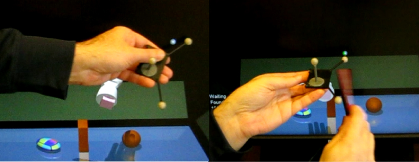
Another test we applied was to tap the hand tracking body with a pen (right panel), record with a 120Hz camera, and count the video frames separating the physical contact event and the change in virtual marker speed (which was printed on the screen in an internal diagnostic mode). Similarly, we moved the physical marker up and down across a horizontal line, and counted the video frames between the physical and virtual markers crossing the line. The latter two tests showed around 42 msec overall latency, and the frame counts were very consistent (5 frames in almost all cases).

Note that these results are obtained with stereoscopic rendering disabled from the NVidia control panel. Enabling it adds some latency. The exact cause of the latency is not yet clear. The Info box in the simulator has a Mocap field that shows the total amount of time that motion capture data spends in the MuJoCo pipeline: from the time it is delivered by the OptiTrack driver to the time the video driver reports that rendering is finished. This time fluctuates between 6 msec and 12 msec, because the relative timing of the OptiTrack and video card fluctuate. This includes processing of the motion capture data, simulation and rendering. The rest is due to latency in the hardware devices we are using, and is higher than what would be expected based on the hardware specifications.

Overall, the virtual environment in MuJoCo HAPTIX is very responsive and usable.

HAPTIX models

MuJoCo HAPTIX is distributed with two models of state-of-the-art prosthetic hands: the Modular Prosthetic Limb (MPL) hand from the Applied Physics Laboratory at Johns Hopkins University, and the Luke hand from DEKA Research. The models have been designed and fine-tuned by Roboti LLC based on information, mesh files and feedback provided by the device manufacturers, as well as testing and feedback from DARPA, the FDA and the performer teams in the DARPA HATPIX program. These simulation models are being used by researchers developing new neural interfaces, which aim to enable amputees to control and sense the next generation of prosthetic hands.

The model of the MPL hand is included in the software distribution and is available to the general public. The model of the Luke hand and its documentation is hosted by DEKA Research and is currently only available to DARPA performer teams. Both models are in MuJoCo's XML file format which is documented in the Modeling chapter.

MPL hand

The MPL hand is the most elaborate prosthetic hand currently available. It has 22 hinge joints in the wrist and hand, driven by 13 motors that can be controlled independently. It also has rich sensing capabilities including joint position and velocity sensors, motor position, velocity and force sensors, and IMUs in each fingertip. The MuJoCo model includes all of the above, plus a number of touch sensors which do not yet exist on the physical device.

MPL joints

The image below shows the position and orientation of the 22 hinge joints as well as the 13 motors. This image can be re-created by loading the model and adjusting the following settings in the Render dialog:

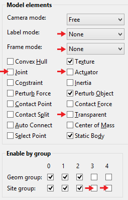
The polarity of each joint and motor is determined by the right-hand rule: if you imagine your right thumb pointing along the arrow, then flexing your fingers corresponds to the positive direction of motion. Each joint and motor is labeled with its name as defined in the XML model file. These names can also be seen in the Sliders dialog. The joints dialog only shows scalar joints (hinge or slide) and not free joints or ball joints. The MPL model uses a combination of free and hinge joints. There is a free joint at the base of the robot model (rendered as a cube) and also in the center of every movable object in the environment.

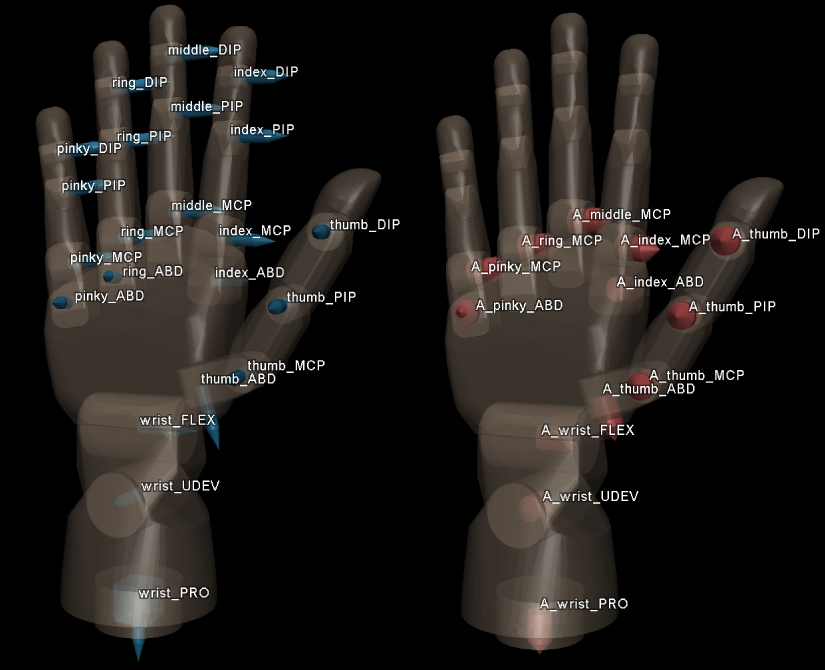
MPL motors

The MPL uses position servos. The user can set the reference positions and feedback gains of these servos at each update cycle, via the socket API described below.

There are fewer motors than joints. Some of the motors (namely wrist, thumb, and index adduction-abduction) are in one-to-one correspondence with a joint. The remaining motors act on multiple joints. In particular, A_pinky_ABD moves both the pinky and ring fingers in the abduction direction. A_index_MCP, A_middle_MCP, A_ring_MCP and A_pinky_MCP move all three joints of the corresponding finger. The physical robot uses elaborate mechanical coupling to implement this distributed action of the motors. In the model, each shared motor drives one of the joints directly (the one with the matching name), and we use equality constraints to passively couple the remaining joints. These constraints are made explicit in the XML model file.

The ordering of the motors in the model corresponds to the order in which the user must provide control signals via the socket API. The table below is from the <actuator> section which can be found towards the end of the XML file.

<actuator>
    <position name="A_wrist_PRO"  joint="wrist_PRO"  ctrlrange="-1.57 1.57"/>
    <position name="A_wrist_UDEV" joint="wrist_UDEV" ctrlrange="-0.26 0.79"/>
    <position name="A_wrist_FLEX" joint="wrist_FLEX" ctrlrange="-1 1"/>
    <position name="A_thumb_ABD"  joint="thumb_ABD"  ctrlrange="0 2.1"/>
    <position name="A_thumb_MCP"  joint="thumb_MCP"  ctrlrange="0 1.0"/>
    <position name="A_thumb_PIP"  joint="thumb_PIP"  ctrlrange="0 1.0"/>
    <position name="A_thumb_DIP"  joint="thumb_DIP"  ctrlrange="-0.82 1.3"/>        
    <position name="A_index_ABD"  joint="index_ABD"  ctrlrange="0 0.34"/>
    <position name="A_index_MCP"  joint="index_MCP"  ctrlrange="0 1.6"/>
    <position name="A_middle_MCP" joint="middle_MCP" ctrlrange="0 1.6"/>
    <position name="A_ring_MCP"   joint="ring_MCP"   ctrlrange="0 1.6"/>
    <position name="A_pinky_ABD"  joint="pinky_ABD"  ctrlrange="0 0.34"/>
    <position name="A_pinky_MCP"  joint="pinky_MCP"  ctrlrange="0 1.6"/>
</actuator>

MPL sensors

The MPL model generates simulated sensor data available via the socket API. There are seven types of sensors:

Joint positions
Joint velocities
Motor positions
Motor velocities
Motor torques
Contact sensors
Inertial measurement unit (IMU) sensors

The joint and motor sensors measure the obvious quantities, in standard units. Recall that motors and joints are not in one-to-one correspondence, which is why it makes sense to have separate joint and motor sensors for position and velocity. The motor torque sensor reflects the internal simulation of a servo motor. In principle this is redundant because the user could have computed the same quantity given the motor position, velocity and command parameters, but is provided for convenience.

IMU sensors measure linear acceleration (in m/s^2) and angular velocity (in rad/s), expressed as 3D vectors in the local coordinate frame of the IMU. The magnitude of the rotation vector corresponds to the speed of rotation, while its direction corresponds to the axis of rotation (using the right-hand rule). Alternatively, one can think of the components of this vector as the amount of instantaneous rotation around each axis of the local frame. The acceleration vector includes gravity. The orientations of the IMU frames relative to the hand segments are shown in the right panel below; the convention is x-red, y-green, z-blue. The x-axis of the local frame points towards the fingernail, the z-axis points along the finger, and the y-axis points to the side (so that together they form right-handed coordinate frame).

Contact sensors are modeled as ellipsoidal sensor zones shown in the image below. Note that the MuJoCo sites defining these zones are in site group #3 which is hidden by default; it can be revealed from the Render dialog. The "palm_back" sensor is on the back of the palm; it appears in the image because text labels are printed on top of the 3D rendering. The simulator detects all contact points that fall within a given sensor zone and involve the body to which the sensor is attached. The contact normal forces of all detected contact points are then added up (as scalars and not vectors) and the result is returned as the output of the simulated contact sensors. Thus the sensor units are Newtons. The sensor output cannot be negative because contact forces cannot pull. As with all other model elements, the sensors are defined in the XML. The complete list of sensors is at the end of the file in the <sensor> section.

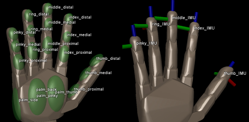
MPL summary table

Below is a summary table of all joints, sensors and actuators defined in the model and their ordering, as exposed in the API. Note that we list sensorized joints and motors only once, even though each joint has a position and velocity sensor attached to it, and each motor has a position, velocity and torque sensor attached to it.

Joint # Joint name Motor # Motor name

0 wrist_PRO 0 A_wrist_PRO

1 wrist_UDEV 1 A_wrist_UDEV

2 wrist_FLEX 2 A_wrist_FLEX

3 thumb_ABD 3 A_thumb_ABD

4 thumb_MCP 4 A_thumb_MCP

5 thumb_PIP 5 A_thumb_PIP

6 thumb_DIP 6 A_thumb_DIP

7 index_ABD 7 A_index_ABD

8 index_MCP 8 A_index_MCP

9 index_PIP

10 index_DIP

11 middle_MCP 9 A_middle_MCP

12 middle_PIP

13 middle_DIP

14 ring_ABD

15 ring_MCP 10 A_ring_MCP

16 ring_PIP

17 ring_DIP

18 pinky_ABD 11 A_pinky_ABD

19 pinky_MCP 12 A_pinky_MCP

20 pinky_PIP

21 pinky_DIP

Contact # Contact name IMU # IMU name

0 palm_thumb

1 palm_pinky

2 palm_side

3 palm_back

4 thumb_proximal

5 thumb_medial

6 thumb_distal 0 thumb_IMU

7 index_proximal

8 index_medial

9 index_distal 1 index_IMU

10 middle_proximal

11 middle_medial

12 middle_distal 2 middle_IMU

13 ring_proximal

14 ring_medial 3 ring_IMU

15 ring_distal

16 pinky_proximal

17 pinky_medial 4 pinky_IMU

18 pinky_distal

Luke hand

The model of the Luke hand is currently only available to performer teams in the DARPA HATPIX program, and is hosted by DEKA Research. The teams should have received instructions how to access that model.

Socket API

MuJoCo HAPTIX can be controlled programmatically over a TCP/IP socket connection. The user program can be executed on the simulation computer or on a different computer running Windows. The API has two flavors: simple and native. It is accessible from C/C++ and from MATLAB. All four combinations are supported. In the following sections we document the API according to flavor (simple vs native), and then for each API function we describe both the C/C++ and MATLAB calling conventions in the same paragraph. As for data structures, we only define the C/C++ versions because the MATLAB versions are identical, with two exceptions: all numeric data fields in MATLAB are double, and all arrays have model-specific size as opposed to a maximum pre-defined size.

Simple vs Native

The simple API was designed in collaboration with the Open Source Robotics Foundation (OSRF) and DARPA, and is intended for use in the DARPA HAPTIX program. It is common to MuJoCo HAPTIX and Gazebo HAPTIX, allowing the same user code to interact with either simulator. This API is adapted to the context of simulating prosthetic hands and is optimized for ease of use. It makes certain assumptions about the model structure. All relevant functions and type definitions are prefixed with hx.

The native API allows more complete access to the simulator, and does not make assumptions about the model structure. This API provides a superset of the functionality accessible via the simple API. All relevant functions and type definitions are prefixed with mj.

An important difference between the two API flavors is how the sizes of variable-size arrays are determined. In the simple API, the user must call the function hx_robot_info which saves the resulting hxRobotInfo data structure internally. Subsequent API calls use the size parameters in this data structure to determine the appropriate array sizes. In contrast, the native API has all necessary size parameters replicated in each data structure containing variable-size arrays. This makes the native API stateless, except for maintaining the socket connection. It also has a mj_info function, similar to hx_robot_info, but calling this function before making other function calls is not strictly required.

Both API flavors are implemented in the same communication libraries, and can be mixed in the same user program.

C/C++ vs MATLAB

The software distribution contains the necessary communication libraries for C/C++ and for MATLAB, in directories "apicpp" and "apimex" respectively. To use the C/C++ API, include "haptix.h" in your code and link with the stub library "mjhaptix_user.lib" which will in turn load the actual library "mjhaptix_user.dll" at runtime. To use the MATLAB API, add the directory "apimex" to the MATLAB path. Note however that the simple flavor of the MATLAB API is common to MuJoCo and Gazebo, thus the corresponding .m files have the same names and calling conventions. If you are installing the API for both simulators on the same machine, be careful to set the path to the simulator you want to work with.

The MATLAB API is a straightforward adaptation of the C/C++ API. Its software architecture however is somewhat unusual from a MATLAB perspective. The C/C++ API is contained in a single dynamic library. In contrast, the usual mode of operation in MATLAB would be to have a separate .m or .mex file for each API function. The problem with the latter approach is that we are using a TCP/IP socket connection, which is established at the beginning of the session and then needs to be maintained. Such maintenance is difficult to achieve if we were to use separate .m or .mex files for each API function, especially since the socket handle created in the underlying C++ code is not a valid MATLAB object. One way around this is to rely on MATLAB's native Java sockets instead - which we have used previously, but they have proven to be slower and less reliable compared to our C++ implementation.

Thus the MATLAB API to MuJoCo HAPTIX is based on a single mex file "mjhx.mexw64". This file automatically locks itself within the MATLAB workspace when a connection to the simulator is established, and automatically unlocks itself when the connection is closed. The user can call it directly (as summarized in the built-in help) but we also provide .m wrappers matching the C/C++ syntax to the extent possible.

Unlike the C/C++ API where most functions return success or error codes, in the MATLAB API errors are generated using MATLAB's standard error handling mechanism, i.e. error messages are printed in the command window and the function terminates.

Simple API reference

The simple API is centered around the hx_update function. This function sends the hxCommand data structure with motor commands to the simulator, and receives the hxSensor data structure with sensor data from the simulator. In MuJoCo this is a blocking call, which returns after a delay corresponding to the update rate specified in the robot model. In Gazebo this is a non-blocking call, but it still returns sensor data that is appropriately delayed. To emulate MuJoCo's approach when using Gazebo, insert a sleep command after the update call. To emulate Gazebo's approach when using MuJoCo, run the update loop in a separate thread.

Before describing the API in detail, we provide a simple example. It is a minimal program that connects to the simulator running on the local host, gets robot info and sensor data, and closes the connection.

#include "haptix.h"

hxRobotInfo info;
hxSensor sensor;

int main(void)
{
    hx_connect(0, 0);
    hx_robot_info(&info);
    hx_read_sensors(&sensor);
    hx_close();
    return 0;
}

A more elaborate and functionally useful example can be found in the file "grasp.cpp" available in the software distribution in the "apicpp" directory. It is designed to work with the MPL model, and implements a grasp reflex using the simulated sensors. Hand closing is initiated when the net contact force reported by the contact sensors exceeds a threshold. The motion is interpolated over 0.5 seconds. The postural target for closing is chosen as the position 2/3 of the way between the lower and upper limit for each motor, where the limits are obtained programmatically through the API. Hand opening is triggered when the net angular velocity reported by the IMUs exceeds a threshold; this requires a flick of the hand. A state machine is used to avoid transitions shorter than 2 seconds. This code uses both the simple and native APIs, but most of the work is done via the simple API. Error checking is left as an exercise for the user.

Restrictions

The simple API makes assumptions about the model structure, both in terms of sensing and in terms of actuation. If these assumptions are violated, API calls will either return errors or the results will not make physical sense. The native API on the other hand supports all valid MuJoCo models.

In term of actuation, only position servos and velocity servos are supported. Furthermore the model is expected to have servos of a single type. The API code checks the first servo, and treats all other servos as having the same type. For position servos, the "ref_pos" command field described later sets the reference position while "gain_pos" sets the position gain. If "ref_vel" is also enabled, it is interpreted as the velocity of the reference position of the servo, and is integrated over a time period corresponding to the API update rate. The latter mechanism is used to emulate positions servos with velocity-like interface. For true velocity servos, "ref_vel" sets the reference velocity and "gain_vel" the velocity gain, while "ref_pos" and "gain_pos" are ignored.

Note that the default actuator gains are specified in the XML model: parameters "kp" and "kv" for position and velocity gains respectively. The user can modify these gains online via the simple API, but this should be done with caution because large gains can lead to instability.

In terms of sensing, the simple API supports joint position and velocity sensors; motor position, velocity and force sensors; touch sensors; IMU sensors. The number of "joints" returned by the simple API does not equal the actual number of joints, but rather the number of joint position or joint velocity sensors, whichever is larger. If both types of sensors are present, their outputs are returned in the order in which they appear in the model. If no joint sensors are present, the number of joints returned by the simple API is 0.

MuJoCo provides accelerometer and gyroscope sensors instead of unified IMU sensors. In contrast, the simple API has a concept of an IMU sensor. This is implemented as follows. The number of IMU sensors returned by the simple API equals the number of accelerometers or gyroscopes, whichever is larger. If both types of sensors are present, their outputs are returned in the order in which they appear in the model. Thus the simple API assumes a model where accelerometers and gyroscopes are defined in pairs, with the two sensors in each pair attached to the same site.

In summary, the ease of use in the context of the DARPA HATPIX program and compatibility with Gazebo provided by the simple API come at the price of significant restrictions. Therefore for general use we recommend the native API.

Data structures

The simple API defines data structures that hold the motor commands and sensor data involved in each update, as well as information about the model. The sizes of the data arrays are determined by the symbols

#define hxMAXMOTOR              32
#define hxMAXJOINT              32
#define hxMAXCONTACTSENSOR      32
#define hxMAXIMU                32

Connecting to the simulator when a larger model is loaded will result in an error message. These sizes are chosen to fit the prosthetic limbs which are the focus of the HAPTIX program.

hxResult

typedef enum
{
    hxOK = 0,                               // success
    hxERROR                                 // error
} hxResult;

This is the type of the result returned by most simple API calls. Note that hxERROR could mean many things; call hx_last_result for a text description of the error. The reason for this implementation (as opposed to enumerating the possible errors directly in hxResult) is because different simulators generate different errors.

hxTime

struct _hxTime
{
    int sec;                                // seconds
    int nsec;                               // nanoseconds
};
typedef struct _hxTime hxTime;

This structure is part of hxSensor below. It represents simulation time rather than system time. In particular, the time resets to 0 when the simulation is reset or a model is loaded or re-loaded. It also pauses when the simulation is paused. The time shown in the info text box in the simulator is identical to the value returned in this structure.

Despite the appearance of a nanosecond clock, there is no such clock here. The "official" simulation time is maintained by the underlying physics engine as a double-precision scalar. This scalar is sent over the socket to the user-side communication library, which then converts it to hxTime. The latter can be converted to double using the function hx_double_time.

Note that this structure does not have a MATLAB equivalent. Instead the MATLAB API returns time as double (in seconds).

hxRobotInfo

struct _hxRobotInfo
{
    // array sizes
    int motor_count;                        // number of motors
    int joint_count;                        // number of hinge joints
    int contact_sensor_count;               // number of contact sensors
    int imu_count;                          // number of IMUs

    // model parameters
    float motor_limit[hxMAXMOTOR][2];       // minimum and maximum motor positions (motor units)
    float joint_limit[hxMAXJOINT][2];       // minimum and maximum joint angles (rad)
    float update_rate;                      // update rate supported by the robot (Hz)
};
typedef struct _hxRobotInfo hxRobotInfo;

This structure contains a (small) subset of the data available in the model description loaded by the simulator. We have selected the fields that are most likely to be useful. After hxRobotInfo is obtained by calling hx_robot_info it should be treated as constant. Changes to it will not be propagated back to the simulator.

The parameter update_rate determines how long the simulator will wait before returning from an update call. The limits for joints and motors are loaded from the XML model. These limits can also be seen in the Sliders dialogs in the simulator.

Recall that the size of the allocated data arrays is 32, while the actual number of elements of each type is smaller - as given by the count fields of hxRobotInfo. When calling the update function, the number of commands you are expected to fill out is motor_count. Similarly when receiving sensor data, the number of fields you should access is the corresponding count. The simulator does not have a mechanism to check if you are aware of these counts; this is your responsibility.

hxSensor

struct _hxSensor
{
    // simulation time
    hxTime time_stamp;                      // simulation time at which the data was collected

    // motor data
    float motor_pos[hxMAXMOTOR];            // motor position (motor-specific units)
    float motor_vel[hxMAXMOTOR];            // motor velocity
    float motor_torque[hxMAXMOTOR];         // motor torque

    // joint data
    float joint_pos[hxMAXJOINT];            // joint position (rad)
    float joint_vel[hxMAXJOINT];            // joint velocity (rad/s)

    // contact data
    float contact[hxMAXCONTACTSENSOR];      // sum of contact normal forces within the sensor zone (N)

    // inertial measurement unit (IMU) data
    float imu_linear_acc[hxMAXIMU][3];      // linear acceleration in IMU frame (m/s^2)
    float imu_angular_vel[hxMAXIMU][3];     // angular velocity in IMU frame (rad/s)
    float imu_orientation[hxMAXIMU][4];     // IMU orientation quaternion; reserved for future use
};
typedef struct _hxSensor hxSensor;

This structure contains all the information returned by the simulator during an update call. The time structure is as discussed above. The motor position and velocity are functions of the joint position and velocity, determined by the mechanical coupling defined in the model. Similarly, the motor torque generated by the servo (and returned in hxSensor) maps to joint torque through the motor moment arm vector, i.e. the vector of partial derivatives of motor position with respect to joint positions. The simulator computes this quantity internally but does not expose it through the API.

The joint position and velocity are part of the state of the 2nd-order system being simulated. The full state also includes the position and velocity of all floating bodies (including the base of the robot) which are not available as sensors. Note that MuJoCo simulates multi-joint dynamics in joint coordinates, in contrast to gaming engines (including ODE which is used in Gazebo) which simulate dynamics in over-complete Cartesian coordinates and impose joint constraints numerically. As a result, the joint positions and velocities returned by MuJoCo are exact.

Contact sensors are modeled via sensor zones that can be visualized in the simulator. Each zone is represented as either ellipsoid or box. At runtime, every contact point that lies within this ellipsoid and is assigned to the sensor's body is included. The contact normal forces of all included contact points are added (as scalars, not vector) and are returned as the simulated output of the contact sensor.

Inertial measurement units (IMUs) are simulated by computing the angular velocity and linear acceleration of the IMU body, and expressing them in the local body frame. In the XML model file the accelerometer and gyroscope sensors are actually defined separately, but the simple API combines them into one IMU sensor. MuJoCo uses a continuous-time formulation (as opposed to a velocity-stepping scheme as is common in gaming engines) and therefore the IMU output is computed analytically. Note that gravity affects the acceleration reading, as with physical IMUs. Some more advanced IMUs have filters that can integrate information over time and estimate a global orientation. We have reserved a field for such data, but are not currently using it because the prosthetic devices we aim to simulate are unlikely to have such sensors. Thus imu_orientation is currently set to (1,0,0,0). The quaternion format we are using is (w,x,y,z).

hxCommand

struct _hxCommand
{
    // servo controller reference values
    float ref_pos[hxMAXMOTOR];              // reference position
    int ref_pos_enabled;                    // should ref_pos be updated in this call
    float ref_vel[hxMAXMOTOR];              // reference velocity
    int ref_vel_enabled;                    // should ref_vel be updated in this call

    // servo controller gains
    float gain_pos[hxMAXMOTOR];             // position feedback gain
    int gain_pos_enabled;                   // should gain_pos be updated in this call
    float gain_vel[hxMAXMOTOR];             // velocity feedback gain
    int gain_vel_enabled;                   // should gain_vel be updated in this call
};
typedef struct _hxCommand hxCommand;

This structure holds all motor commands sent to the simulator. The xxx_enabled flags specify if the corresponding command data should be updated in this call. Positive values mean enabled, zero or negative values mean disabled. Make sure to disable all fields that you do not intend to update. The gains in particular would normally be left to their default settings or updated only occasionally (unless you are experimenting with some form of impedance control). As specified in the Servo control description, the velocity references and gains are ignored for now. It is your responsibility to fill out the correct number of motor commands (which is hxRobotInfo.motor_count) in each array.

Functions

The API functions provide a way to exchange the above data structures with the simulator. Thus the main part of the documentation is in the data structure description. Note that error checking is the responsibility of the user. When the result returned by any function is hxERROR (instead of the desirable hxOK), the most straightforward action is to print out the string returned by hx_last_result and exit. Continuing the execution of the regular code will simply yield more hxERRORs.

All API functions assume that MuJoCo HAPTIX has been started and a model has been loaded. If this is not the case you will get an error. Calling the API functions when the simulation is paused is not an error, but the motor commands will not have any effect.

The calling convention for each function is specified both for the C/C++ API and for the MATLAB API, denoted with "C:" and "M:" respectively.

hx_connect

C: hxResult hx_connect(const char* host, int port);
M: function hx_connect(host, port)

Establish socket connection to the simulator. The port argument is ignored in MuJoCo (since we use a fixed port) and is provided for compatibility with Gazebo. If the user code is running on the simulation computer, set host to NULL (in C only) or pass the empty string to specify the local host. Do not use "localhost" or "127.0.0.1". When using a remote computer, host must be a string with either the name or IP address of the simulation computer.

The simulator shows the status of the socket connection in the info text box. It can be "Waiting" or "Connected". Only one client can connect to the simulator.

hx_close

C: hxResult hx_close(void);
M: function hx_close

Close the previously established connection to the simulator. If the user program exits without calling this function, the simulator will detect that the socket is broken and close it on its end, and go back to waiting mode. But hx_close is the clean way to terminate a connection.

hx_robot_info

C: hxResult hx_robot_info(hxRobotInfo* robotinfo);
M: function info = hx_robot_info

The C/C++ API returns the hxRobotInfo structure described above. The MATLAB API returns the equivalent structure:

   info = 
                motor_count: 13
                joint_count: 22
       contact_sensor_count: 19
                  imu_count: 5
                motor_limit: [13x2 double]
                joint_limit: [22x2 double]
                update_rate: 50

This function not only provides useful information to the user, but also saves the result internally and later uses it to determine the sizes of the variable-size arrays in hxSensor and hxCommand. Thus it nust be called when the connection to the simulator is first established, and when a different model is loaded.

hx_update

C: hxResult hx_update(const hxCommand* command, hxSensor* sensor);
M: function sensor = hx_update(command)

This is the main update function. It returns after 1000/update_rate ms. If update_rate is less than 1, it returns at the maximum speed supported by the TCP/IP connection. See the descriptions of hxCommand and hxSensor. Note that calling this function when the simulation is paused still sets the controls signals, but has no other effect. In contrast, the corresponding function mj_update in the native API sets the control signals and calls the internal step function, thereby advancing the simulation by one timestep when paused.

For the MATLAB API, you have to construct the command structure directly using the struct command in MATLAB. The sensor structure is returned to you. These structures have the form:

   command = 
                   ref_pos: [13x1 double]
               ref_vel_max: [13x1 double]
                  gain_pos: [13x1 double]
                  gain_vel: [13x1 double]
           ref_pos_enabled: 1
       ref_vel_max_enabled: 0
          gain_pos_enabled: 0
          gain_vel_enabled: 0

   sensor = 
            time_stamp: 20.05
             motor_pos: [13x1 double]
             motor_vel: [13x1 double]
          motor_torque: [13x1 double]
             joint_pos: [22x1 double]
             joint_vel: [22x1 double]
               contact: [19x1 double]
        imu_linear_acc: [5x3 double]
       imu_angular_vel: [5x3 double]
       imu_orientation: [5x4 double]

hx_read_sensors

C: hxResult hx_read_sensors(hxSensor* sensor);
M: function sensor = hx_read_sensors

This is a light version of hx_update where the command is not updated but the sensor data is still returned. It has the same blocking behavior as hx_update. In fact it is implemented internally as a call to hx_update, with a dummy hxCommand argument whose xxx_enabled flags are all set to 0.

hx_last_result

C: const char* hx_last_result(void);
M: n/a

This function returns a text description of the last result returned by any API call. Even though the functions in the simple API return a generic hxOK or hxERROR code to the user, the actual error code is saved internally, and is then translated into text using this function.

hx_double_time

C: double hx_double_time(const hxTime* time);
M: n/a

This function converts the sec:nsec time representation in hxTime to a double, expressed in seconds. It does not call the simulator. Call it with a pointer to the hxTime structure returned as part of hxSensor.

Native API reference

The native API involves a substantially larger number of data structures and functions compared to the simple API. This is because the native API is designed to be more powerful and provide more direct access to the simulator (but is still limited compared to the shared-memory API available in MuJoCo Pro). This more direct access requires some understanding of how MuJoCo works internally. The present section provides some of the necessary information, but it cannot replace the preceding chapters explaining in detail how the simulator works.

In the context of the DARPA HAPTIX program, the Simple API should be used to control the robot while the Native API should be used for everything else - moving objects, changing colors, computing scoring functions etc. In this context the Native API can also be thought of as a "World API". Note that the Gazebo HAPTIX simulator also has a World API, which is not compatible but is designed to enable similar functionality. In more general scenarios however we recommend using only the Native API, including for controlling robots. This is because the Simple API assumes a position-controlled robot with certain arrangement of sensors, and is not compatible with more general robot models.

Perhaps the most important thing to keep in mind about MuJoCo is that it operates in generalized or joint coordinates, unlike gaming engines (such as ODE, Bullet, Havoc, PhysX) which operate in Cartesian coordinates and which provide the simulation capability in packages such as Gazebo and V-Rep. The consequences of this are explained in the Joint coordinates section of the Overview chapter.

Another important consideration are the different types of model elements that MuJoCo supports and that are exposed via the native API. They can be summarized as follows:

The vectors "qpos" and "qvel" contain the 2nd-order system state in terms of generalized position and velocity. If there are actuators with activation dynamics in the model (e.g. muscles or pneumatic cylinders), then the vector "act" also becomes part of the system state. The state is exposed in mjState;
Actuators are abstract entities that receive a scalar input, somehow map it to a scalar force, which is then mapped to joint torques via a transmission model. The control vector "ctrl" contains all actuator inputs and is exposed in mjControl. Information about actuators is exposed in mjActuator;
Tendons can be spatial tendons modeled as minimal-length paths that wrap around specified obstacles, or fixed combinations of joint angles. Information about tendons is exposed in mjTendon;
Bodies have mass, inertia matrix, and spatial frame attached to them (whose position and orientation is computed via forward kinematics). Geoms and sites also have spatial frames, but they are attached to a body and always move with it. Multiple geoms and sites can be attached to the same body. Kinematic information about all bodies, geoms and sites is exposed in mjBody, mjGeom and mjSite;
Mocap bodies are special: they are stationary as far as the physics model is concerned (i.e. they are defined as children of the world body without any joints), but at each time step their position and orientation can change based on mocap data exposed in mjMocap;
The dynamics are defined in continuous-time as: inertia * acceleration + bias = applied + passive + actuator + constraint. The generalized inertia matrix is computed internally and cannot be accessed via the socket API. The generalized force vectors "bias", "applied", "passive", "actuator" and "constraint" are exposed in mjForce. The generalized acceleration (which is the main output of the forward dynamics) is exposed in mjDynamics;
The constraint solver in MuJoCo (which is responsible for computing the generalized constraint force) treats contacts, equality constraints, joint and tendon limits, and dry friction in joints and tendons in a unified framework. Information about all active contacts is exposed in mjContact;
Sensors defined in the model are used to construct an array of sensor data exposed in mjSensor. This array can be decoded using the sensor specifications exposed in mjInfo.

Codes

The integer constants defined here are needed to interpret the error codes and the types of various MuJoCo objects.

mjtResult

typedef enum
{
    mjCOM_OK            = 0,            // success

// server-to-client errors
    mjCOM_BADSIZE       = -1,           // data has invalid size
    mjCOM_BADINDEX      = -2,           // object has invalid index
    mjCOM_BADTYPE       = -3,           // invalid object type
    mjCOM_BADCOMMAND    = -4,           // unknown command
    mjCOM_NOMODEL       = -5,           // model has not been loaded
    mjCOM_CANNOTSEND    = -6,           // could not send data
    mjCOM_CANNOTRECV    = -7,           // could not receive data
    mjCOM_TIMEOUT       = -8,           // receive timeout

    // client-side errors
    mjCOM_NOCONNECTION  = -9,           // connection not established
    mjCOM_CONNECTED     = -10,          // already connected
} mjtResult;

Unlike the simple API where function calls return the generic error code hxERROR which is then decoded via hx_last_result, here function calls return specific error codes. If you want to print the associated error string, you can still call hx_last_result. This works because the last error is always saved internally, regardless of which API flavor was used.

mjtGeom

typedef enum
{
    mjGEOM_PLANE = 0,                   // plane
    mjGEOM_HFIELD,                      // height field
    mjGEOM_SPHERE,                      // sphere
    mjGEOM_CAPSULE,                     // capsule
    mjGEOM_ELLIPSOID,                   // ellipsoid
    mjGEOM_CYLINDER,                    // cylinder
    mjGEOM_BOX,                         // box
    mjGEOM_MESH                         // mesh
} mjtGeom;

Type of geometric shape (or geom) used for visualization and collision detection. This can be used to decode mjInfo.geom_type.

mjtSensor

typedef enum             
{
    // common robotic sensors, attached to a site
    mjSENS_TOUCH        = 0,            // scalar contact normal forces summed over sensor zone
    mjSENS_ACCELEROMETER,               // 3D linear acceleration, in local frame
    mjSENS_VELOCIMETER,                 // 3D linear velocity, in local frame
    mjSENS_GYRO,                        // 3D angular velocity, in local frame
    mjSENS_FORCE,                       // 3D force between site's body and its parent body
    mjSENS_TORQUE,                      // 3D torque between site's body and its parent body
    mjSENS_MAGNETOMETER,                // 3D magnetometer
    mjSENS_RANGEFINDER,                 // scalar distance to nearest geom or site along z-axis

    // sensors related to scalar joints, tendons, actuators
    mjSENS_JOINTPOS,                    // scalar joint position (hinge and slide only)
    mjSENS_JOINTVEL,                    // scalar joint velocity (hinge and slide only)
    mjSENS_TENDONPOS,                   // scalar tendon position
    mjSENS_TENDONVEL,                   // scalar tendon velocity
    mjSENS_ACTUATORPOS,                 // scalar actuator position
    mjSENS_ACTUATORVEL,                 // scalar actuator velocity
    mjSENS_ACTUATORFRC,                 // scalar actuator force

    // sensors related to ball joints
    mjSENS_BALLQUAT,                    // 4D ball joint quaterion
    mjSENS_BALLANGVEL,                  // 3D ball joint angular velocity

    // sensors attached to an object with spatial frame: (x)body, geom, site, camera
    mjSENS_FRAMEPOS,                    // 3D position
    mjSENS_FRAMEQUAT,                   // 4D unit quaternion orientation
    mjSENS_FRAMEXAXIS,                  // 3D unit vector: x-axis of object's frame
    mjSENS_FRAMEYAXIS,                  // 3D unit vector: y-axis of object's frame
    mjSENS_FRAMEZAXIS,                  // 3D unit vector: z-axis of object's frame
    mjSENS_FRAMELINVEL,                 // 3D linear velocity
    mjSENS_FRAMEANGVEL,                 // 3D angular velocity
    mjSENS_FRAMELINACC,                 // 3D linear acceleration
    mjSENS_FRAMEANGACC,                 // 3D angular acceleration

    // sensors related to kinematic subtrees; attached to a body (which is the subtree root)
    mjSENS_SUBTREECOM,                  // 3D center of mass of subtree
    mjSENS_SUBTREELINVEL,               // 3D linear velocity of subtree
    mjSENS_SUBTREEANGMOM,               // 3D angular momentum of subtree

    // user-defined sensor
    mjSENS_USER                         // sensor data provided by mjcb_sensor callback
} mjtSensor;

Type of sensor. This can be used to decode mjInfo.sensor_type. See the documentation of mjInfo for more details on how to interpret the sensor data array.

Touch sensors are modeled via sensor zones that can be visualized in the simulator. Each zone is represented as either ellipsoid or box. At runtime, every contact point that lies within this ellipsoid/box and is assigned to the sensor's body is included. The contact normal forces of all included contact points are added (as scalars, not vectors) and are returned as the scalar output of the contact sensor.

Inertial measurement units (IMUs) are simulated by computing the angular velocity and linear acceleration of the IMU body, and expressing them in the local body frame. MuJoCo uses a continuous-time formulation of physics and therefore the IMU output is computed analytically. Note that gravity affects the acceleration reading, as with physical IMUs. The IMU sensor outputs 6 scalars: 3 angular velocities followed by 3 linear accelerations.

Six-axis force-torque sensors (FT) measure the interaction force between a body and its parent body,regardless of whether the two bodies are welded or there are joints between them. The FT sensor outputs 6 scalars: 3 linear forces followed by 3 rotational torques. The are all expressed in the local frame of the child body to which the sensor is attached.

See the sensor documentation in the Modeling chapter for more information.

mjtJoint

typedef enum
{
    mjJNT_FREE = 0,                     // "joint" defining floating body
    mjJNT_BALL,                         // ball joint
    mjJNT_SLIDE,                        // sliding/prismatic joint
    mjJNT_HINGE                         // hinge joint
} mjtJoint;

Type of joint. This can be used to decode mjInfo.jnt_type.

Free joints are used to define a floating body. They contribute 7 elements to "qpos": a 3D position followed by a unit quaternion; and 6 elements to "qvel": a 3D linear velocity followed by a 3D angular velocity. This is why "qpos" and "qvel" can have different dimensionality. Ball joints contribute a unit quanterion to "qpos" and a 3D angular velocity to "qvel". Slide and hinge joints are scalar.

mjtTrn

typedef enum
{
    mjTRN_JOINT = 0,                    // force on joint
    mjTRN_JOINTINPARENT,                // force on joint, expressed in parent frame
    mjTRN_SLIDERCRANK,                  // force via slider-crank linkage
    mjTRN_TENDON,                       // force on tendon
    mjTRN_SITE                          // force on site
} mjtTrn;

Type of actuator transmission. This can be used to decode mjInfo.actuator_trntype. For a description of these transmission types, see the general actuator documentation in the Modeling chapter.

mjtEq

typedef enum
{
    mjEQ_CONNECT = 0,                   // connect two bodies at a point (ball joint)
    mjEQ_WELD,                          // fix relative position and orientation of two bodies
    mjEQ_JOINT,                         // couple the values of two scalar joints with cubic
    mjEQ_TENDON,                        // couple the lengths of two tendons with cubic
    mjEQ_DISTANCE                       // fix the contact distance between two geoms
} mjtEq;

Type of equality constraint. This can be used to decode mjInfo.eq_type. Note that in generalized coordinates most joints are represented implicitly via the structure of the kinematic tree. Nevertheless there is sometimes need to add explicit equality constraints and enforce them numerically (e.g. loop joints.)

Connect means that two bodies are connected with a ball joint, i.e. a point local to one body is forced to coincide with a point local to the other body. Weld means that two bodies are welded together and can neither translate nor rotate relative to each other. Joint and tendon mean that two scalar joints or two tendons are coupled via a cubic polynomial. Distance means that the nearest distance between the surfaces of the geoms remains constant.

Data structures

Similar to the simple API, here we define a maximum size for all variable-size arrays and pre-allocate the necessary space when each data structure is created. This avoids repeated memory allocation and deallocation at runtime. The maximum size is:

#define mjMAXSZ  200

If this size is exceeded for a given API call, the error code mjCOM_BADSIZE is returned.

mjInfo

struct _mjInfo
{
    // sizes
    int nq;                             // number of generalized positions
    int nv;                             // number of generalized velocities
    int na;                             // number of actuator activations
    int njnt;                           // number of joints
    int nbody;                          // number of bodies
    int ngeom;                          // number of geoms
    int nsite;                          // number of sites
    int ntendon;                        // number of tendons
    int nu;                             // number of actuators/controls
    int neq;                            // number of equality constraints
    int nkey;                           // number of keyframes
    int nmocap;                         // number of mocap bodies
    int nsensor;                        // number of sensors
    int nsensordata;                    // number of elements in sensor data array
    int nmat;                           // number of materials

    // timing parameters
    float timestep;                     // simulation timestep
    float apirate;                      // API update rate (same as hxRobotInfo.update_rate)

    // sensor descriptors
    int sensor_type[mjMAXSZ];           // sensor type (mjtSensor)
    int sensor_datatype[mjMAXSZ];       // type of sensorized object
    int sensor_objtype[mjMAXSZ];        // type of sensorized object
    int sensor_objid[mjMAXSZ];          // id of sensorized object
    int sensor_dim[mjMAXSZ];            // number of (scalar) sensor outputs
    int sensor_adr[mjMAXSZ];            // address in sensor data array
    float sensor_noise[mjMAXSZ];        // noise standard deviation

    // joint properties
    int jnt_type[mjMAXSZ];              // joint type (mjtJoint)
    int jnt_bodyid[mjMAXSZ];            // id of body to which joint belongs
    int jnt_qposadr[mjMAXSZ];           // address of joint position data in qpos
    int jnt_dofadr[mjMAXSZ];            // address of joint velocity data in qvel
    float jnt_range[mjMAXSZ][2];        // joint range; (0,0): no limits

    // geom properties
    int geom_type[mjMAXSZ];             // geom type (mjtGeom)
    int geom_bodyid[mjMAXSZ];           // id of body to which geom is attached

    // equality constraint properties
    int eq_type[mjMAXSZ];               // equality constraint type (mjtEq)
    int eq_obj1id[mjMAXSZ];             // id of constrained object
    int eq_obj2id[mjMAXSZ];             // id of 2nd constrained object; -1 if not applicable

    // actuator properties
    int actuator_trntype[mjMAXSZ];      // transmission type (mjtTrn)
    int actuator_trnid[mjMAXSZ][2];     // transmission target id
    float actuator_ctrlrange[mjMAXSZ][2]; // actuator control range; (0,0): no limits
};
typedef struct _mjInfo mjInfo;

This is a subset of the information available in the mjModel data structure used in the Pro API. It has several sections as follows.

The size section contains the numbers of various model elements. These integers are also copied in the data structures containing the corresponding variable-size arrays, so as to make the API stateless.

The timing section specifies the simulation timestep used for numerical integration, and the rate at which the socket API can run the mj_update function.

The sensor descriptors are essential for decoding the sensor data array exposed in mjSensor. Each sensor has a type (see mjtSensor above), id of the object to which it is attached, dimensionality (i.e. number of scalar outputs), and 0-based address in the global sensor data array. The type of sensor determines the type of attachment object as well as its dimensionality. For example, if sensor_type[i]==mjSENS_JOINTPOS then the i-th sensor is a joint position sensor, and therefore sensor_objid[i] is the 0-based id of a joint, and sensor_dim[i] is 1 (we include sensor_dim for user convenience.)

The joint section specifies the joint types and the addresses where the corresponding data resides in the global vectors "qpos" and "qvel". Also provided are the id of the (child) body to which the joint belongs, and the joint range if specified in the model.

The geom section specifies the type of each geom and the id of the body to which it is attached.

The equality constraint section specifies the type of each equality constraint and the ids of the objects it couples. The object types are implicitly determined by the equality constraint type.

The actuator section specifies the types of actuator transmission, the id of the object to which the transmission is attached, and the range or acceptable control signals if defined in the model.

mjState

struct _mjState
{
    int nq;                             // number of generalized positions
    int nv;                             // number of generalized velocities
    int na;                             // number of actuator activations
    float time;                         // simulation time
    float qpos[mjMAXSZ];                // generalized positions
    float qvel[mjMAXSZ];                // generalized velocities
    float act[mjMAXSZ];                 // actuator activations
};
typedef struct _mjState mjState;

This is the state of the simulated system in generalized coordinates. Actuators that have their own activations are rare, thus "na" is usually 0.

mjControl

struct _mjControl
{
    int nu;                             // number of actuators
    float time;                         // simulation time
    float ctrl[mjMAXSZ];                // control signals
};
typedef struct _mjControl mjControl;

This is the vector of control signals applied to the actuators.

mjApplied

struct _mjApplied
{
    int nv;                             // number of generalized velocities
    int nbody;                          // number of bodies
    float time;                         // simulation time
    float qfrc_applied[mjMAXSZ];        // generalized forces
    float xfrc_applied[mjMAXSZ][6];     // Cartesian forces and torques applied to bodies
};
typedef struct _mjApplied mjApplied;

User-specified applied forces, in generalized and Cartesian coordinates respectively.

mjOneBody

struct _mjOneBody
{
    int bodyid;                         // body id, provided by user

    // get only
    int isfloating;                     // 1 if body is floating, 0 otherwise
    float time;                         // simulation time
    float linacc[3];                    // linear acceleration
    float angacc[3];                    // angular acceleration
    float contactforce[3];              // net force from all contacts on this body

    // get for all bodies; set for floating bodies only
    //  (setting the state of non-floating bodies would require inverse kinematics)
    float pos[3];                       // position
    float quat[4];                      // orientation quaternion
    float linvel[3];                    // linear velocity
    float angvel[3];                    // angular velocity

    // get and set for all bodies 
    //  (modular access to the same data as provided by mjApplied.xfrc_applied)
    float force[3];                     // Cartesian force applied to body CoM
    float torque[3];                    // Cartesian torque applied to body
};
typedef struct _mjOneBody mjOneBody;

Detailed information about a single body. The user must set bodyid. The function mj_get_onebody fills in all other fields. The function mj_set_onebody sets the fields marked as "set" in the simulator. Note that positions and velocities can only be set for floating bodies.

mjMocap

struct _mjMocap
{
    int nmocap;                         // number of mocap bodies
    float time;                         // simulation time
    float pos[mjMAXSZ][3];              // positions
    float quat[mjMAXSZ][4];             // quaternion orientations
};
typedef struct _mjMocap mjMocap;

The positions and orientations of the mocap bodies. These bodies are defined as static children of the world body. Nevertheless in the forward kinematics stage they can be positioned and oriented - usually to track external data from a motion capture system, but the user can utilize this functionality for other purposes as well.

When using the integrated motion capture functionality in MuJoCo HAPTIX, the position and orientation of the hand-tracking body is copied into mocap body 0, which in the model definition is coupled to the base of the simulated robot with a weld equality constraint. Getting this data structure from the simulator can be used to read the motion capture data. Setting it can be used to move static bodies around (as long as they were defined in the model of course).

mjDynamics

struct _mjDynamics
{
    int nv;                             // number of generalized velocities
    int na;                             // number of actuator activations
    float time;                         // simulation time
    float qacc[mjMAXSZ];                // generalized accelerations
    float actdot[mjMAXSZ];              // time-derivatives of actuator activations
};
typedef struct _mjDynamics mjDynamics;

The main output of the forward dynamics computation. If there are actuator activations in the model, their time-derivative is also included.

mjSensor

struct _mjSensor
{
    int nsensordata;                    // size of sensor data array
    float time;                         // simulation time
    float sensordata[mjMAXSZ];          // sensor data array
};
typedef struct _mjSensor mjSensor;

The sensor data array. See mjtSensor and mjInfo for instructions on how to decode this array.

mjBody

struct _mjBody
{
    int nbody;                          // number of bodies
    float time;                         // simulation time
    float pos[mjMAXSZ][3];              // positions
    float mat[mjMAXSZ][9];              // frame orientations
};
typedef struct _mjBody mjBody;

The positions and orientations of all body frames, as computed by forward kinematics. "mat" is a 3-by-3 orientation matrix in row-major format.

mjGeom

struct _mjGeom
{
    int ngeom;                          // number of geoms
    float time;                         // simulation time
    float pos[mjMAXSZ][3];              // positions
    float mat[mjMAXSZ][9];              // frame orientations
};
typedef struct _mjGeom mjGeom;

The positions and orientations of all geom frames, as computed by forward kinematics.

mjSite

struct _mjSite
{
    int nsite;                          // number of sites
    float time;                         // simulation time
    float pos[mjMAXSZ][3];              // positions
    float mat[mjMAXSZ][9];              // frame orientations
};
typedef struct _mjSite mjSite;

The positions and orientations of all site frames, as computed by forward kinematics.

mjTendon

struct _mjTendon
{
    int ntendon;                        // number of tendons
    float time;                         // simulation time
    float length[mjMAXSZ];              // tendon lengths
    float velocity[mjMAXSZ];            // tendon velocities    
};
typedef struct _mjTendon mjTendon;

The lengths and velocities of all tendons.

mjActuator

struct _mjActuator
{
    int nu;                             // number of actuators
    float time;                         // simulation time
    float length[mjMAXSZ];              // actuator lengths
    float velocity[mjMAXSZ];            // actuator velocities
    float force[mjMAXSZ];               // actuator forces
};
typedef struct _mjActuator mjActuator;

The lengths, velocities of scalar forces of all actuators.

mjForce

struct _mjForce
{
    int nv;                             // number of generalized velocities/forces
    float time;                         // simulation time
    float applied[mjMAXSZ];             // applied/perturbation forces                  
    float passive[mjMAXSZ];             // passive forces                   
    float bias[mjMAXSZ];                // internal and gravitational forces
    float actuator[mjMAXSZ];            // actuator forces                  
    float constraint[mjMAXSZ];          // constraint forces                    
};
typedef struct _mjForce mjForce;

All generalized forces acting on the system.

mjContact

struct _mjContact
{
    int ncon;                           // number of detected contacts
    float time;                         // simulation time
    float pos[mjMAXSZ][3];              // contact position             
    float frame[mjMAXSZ][9];            // contact frame (0-2: normal)  
    float dist[mjMAXSZ];                // normal distance
    float force[mjMAXSZ][3];            // force in contact frame       
    int geom1[mjMAXSZ];                 // id of 1st contacting geom    
    int geom2[mjMAXSZ];                 // id of 2nd contacting geom (force: 1st -> 2nd)
};
typedef struct _mjContact mjContact;

Information about all active contacts. For each contact we include the 3D position of the contact point (i.e. the point in the middle of the shortest line segment connecting the two surfaces), the contact frame, the distance between the two surfaces (negative means penetration), the 3D contact force generated by the constraint solver, and the ids of the two geoms forming the contact. The force is expressed in the contact frame, whose first axis is the contact normal followed by the two tangent axes. Recall that a frame is the transpose of an orientation matrix. Again, MuJoCo matrices have row-major format.

Note that contacts are formed between geoms and not bodies. The same body can have multiple geoms attached to it. To find out the bodies that are involved in contact i, look up mjInfo.geom_bodyid[mjContact.geom1[i]] and similary for geom2. The contact force is directed from geom1 towards geom2.

Functions

All API functions assume that MuJoCo HAPTIX has been started and a model has been loaded. If this is not the case you will get an error. The calling convention for each function is specified both for the C/C++ API and for the MATLAB API, denoted with "C:" and "M:" respectively.

The functions are organized in three categories: get, set, miscellaneous. All get functions return the current simulation time, while the corresponding set functions ignore the time field. There is a large number of get functions and a small number of set functions. This is because most of the get functions correspond to results of the overall computations rather than entry points.

mj_get_state

C: mjtResult mj_get_state(mjState* state);
M: function state = mj_get_state

Get the mjState data structure containing the simulation state.

mj_get_control

C: mjtResult mj_get_control(mjControl* control);
M: function control = mj_get_control

Get the mjControl data structure containing the vector of control signals acting on the actuators.

mj_get_applied

C: mjtResult mj_get_applied(mjApplied* applied);
M: function applied = mj_get_applied

Get the mjApplied data structure containing user-specified applied forces in generalized and Cartesian coordinates.

mj_get_onebody

C: mjtResult mj_get_onebody(mjOneBody* onebody);
M: function onebody = mj_get_onebody(bodyid)

Get the mjOneBody data structure containing detailed information about a single body. Note that the MATLAB function takes the body id as an argument, while the C function expects the user to set onebody->bodyid before the call.

mj_get_mocap

C: mjtResult mj_get_mocap(mjMocap* mocap);
M: function mocap = mj_get_mocap

Get the mjMocap data structure containing the positions and orientations of the mocap bodies defined in the model.

mj_get_dynamics

C: mjtResult mj_get_dynamics(mjDynamics* dynamics);
M: function dynamics = mj_get_dynamics

Get the mjDynamics data structure containing the main output of the forward dynamics.

mj_get_sensor

C: mjtResult mj_get_sensor(mjSensor* sensor);
M: function sensor = mj_get_sensor

Get the mjSensor data structure containing the sensor data array.

mj_get_body

M: mjtResult mj_get_body(mjBody* body);
C: function body = mj_get_body

Get the mjBody data structure containing the positions and orientations of all bodies.

mj_get_geom

C: mjtResult mj_get_geom(mjGeom* geom);
M: function geom = mj_get_geom

Get the mjGeom data structure containing the positions and orientations of all geoms.

mj_get_site

C: mjtResult mj_get_site(mjSite* site);
M: function site = mj_get_site

Get the mjSite data structure containing the positions and orientations of all sites.

mj_get_tendon

C: mjtResult mj_get_tendon(mjTendon* tendon);
M: function tendon = mj_get_tendon

Get the mjTendon data structure containing the lengths and velocities of all tendons.

mj_get_actuator

C: mjtResult mj_get_actuator(mjActuator* actuator);
M: function actuator = mj_get_actuator

Get the mjActuator data structure containing the lengths, velocities and forces of all actuators.

mj_get_force

C: mjtResult mj_get_force(mjForce* force);
M: function force = mj_get_force

Get the mjForce data structure containing all generalized forces acting on the system.

mj_get_contact

C: mjtResult mj_get_contact(mjContact* contact);
M: function contact = mj_get_contact

Get the mjContact data structure containing information about all active contacts.

mj_set_state

C: mjtResult mj_set_state(const mjState* state);
M: function mj_set_state(state)

Set the state of the simulated system. The user is expected to fill out the data structure mjState. The size parameters "nq", "nv" and "na" must match the corresponding sizes of the model being simulated; otherwise error mjCOM_BADSIZE is returned. The correct size parameters can be obtained using mj_get_state or mj_info. The time field is ignored.

For the MATLAB interface, the necessary structure can be created using the struct command:

>> state = struct('nq',7, 'nv',6, 'na',0, 'time',0, 'qpos',zeros(7,1), 'qvel',zeros(6,1), 'act',[])

state = 

      nq: 7
      nv: 6
      na: 0
    time: 0
    qpos: [7x1 double]
    qvel: [6x1 double]
     act: []

mj_set_control

C: mjtResult mj_set_control(const mjControl* control);
M: function mj_set_control(control)

Set the control signals acting on the actuators. The user is expected to fill out the data structure mjControl. The size parameter "nu" must match the corresponding size of the model being simulated; otherwise error mjCOM_BADSIZE is returned.

Setting the control with this function makes sense when the mj_step function will be called next and sensor data is not needed. Otherwise the mj_update function is more efficient because it sends the control signals and receives the sensor data in a single exchange over the socket.

mj_set_applied

C: mjtResult mj_set_applied(const mjApplied* applied);
M: function mj_set_applied(applied)

Set the user-specified applied forces acting on the system. The user is expected to fill out the data structure mjApplied. The size parameters "nu" and "nbody" must match the corresponding sizes of the model being simulated; otherwise error mjCOM_BADSIZE is returned.

The forces specified here are added to the actuator forces. This provides an alternative way to control the simulation when actuators are not present in the model.

mj_set_onebody

C: mjtResult mj_set_onebody(const mjOneBody* onebody);
M: function mj_set_onebody(onebody)

Set the state and forces acting on a single body. The user is expected to fill out the data structure mjOneBody. The parameter "bodyid" must be a valid body id; otherwise error mjCOM_BADINDEX is returned.

For floating bodies, this function sets the position, oriention, linear and angular velocity of the free joint connecting the body to the world. he force and torque are set for all bodies; these correspond to the body-specific elements of the global array xfrc_applied exposed in mjApplied.

mj_set_mocap

C: mjtResult mj_set_mocap(const mjMocap* mocap);
M: function mj_set_mocap(mocap)

Set the positions and orientations of the mocap bodies defined in the model. The user is expected to fill out the data structure mjMocap. The size parameter "nmocap" must match the corresponding size of the model being simulated; otherwise error mjCOM_BADSIZE is returned.

When the integrated motion capture functionality is enabled, the software automatically writes the position and orientation of the hand-tracking body in mocap body 0. Using this function will overwrite the current information and may cause flicker on the screen. This function is useful for moving mocap bodies other than the one being moved automatically by the motion capture system. Thus the recommended usage pattern is to get the mjMocap data, modify the information for bodies other than body 0 as needed, and then set it immediately.

mj_set_geomsize

C: mjtResult mj_set_geomsize(int geomid, const float* geomsize);
M: function mj_set_geomsize(geomid, geomsize)

Sets the size of the specified geom. The size is a vector with 3 elements, even if not all of them are used by this type of geom. See geom in the Modeling chapter for explanation of the geom size convention.

mj_get_rgba

C: mjtResult mj_get_rgba(const char* type, int id, float* rgba);
M: function rgba = mj_get_rgba(type, id)

Returns the rgba field of the specified model element. The type must be one of: "geom", "site", "tendon", "material". If the type or corresponding element id are invalid, the function returns mjCOM_BADTYPE or mjCOM_BADINDEX respectively.

mj_set_rgba

C: mjtResult mj_set_rgba(const char* type, int id, const float* rgba);
M: function mj_set_rgba(type, id, rgba)

Sets the rgba field of the specified model element. The type must be one of: "geom", "site", "tendon", "material". If the type or corresponding element id are invalid, the function returns mjCOM_BADTYPE or mjCOM_BADINDEX respectively.

All elements of the rgba vector are automatically clamped to the range [0, 1]. Setting the alpha (i.e. transparency) component to 0 makes the object invisible.

For model elements that have both material and rgba fields, the material specification takes precedence. Note that materials are often specified via defaults - so you if attempt to set the rgba of a geom and there is no visible effect, that is because a material was already applied to that geom.

mj_connect

C: mjtResult mj_connect(const char* host);
M: function mj_connect(host)

Connect to the simulator. This is equivalent to calling hx_connect except the nuisance port parameter is omitted. Only one of these functions should be called per connection; otherwise the second call with return with error mjCOM_CONNECTED.

mj_close

C: mjtResult mj_close(void);
M: function mj_close

Close the connection to the simulator. This is equivalent to calling hx_close.

mj_result

C: mjtResult mj_result(void);
M: n/a

Return the result from the last API call (which is always saved internally). This function is not available in MATLAB because error messages are printed directly in the command window.

mj_connected

C: int mj_connected(void);
M: function connected = mj_connected

Return 1 if a socket connection to the simulator has been established and is in valid state, and 0 otherwise.

mj_info

C: mjtResult mj_info(mjInfo* info);
M: function info = mj_info

Return the mjInfo data structure describing the current model.

mj_step

C: mjtResult mj_step(void);
M: function mj_step

If the simulation is paused this function will advance it by one time step, sleep for 1 msec, and return. If the simulation is running this function has no effect and returns immediately.

mj_update

C: mjtResult mj_update(const mjControl* control, mjSensor* sensor);
M: function sensor = mj_update(control)

This function sets the control vector similar to mj_set_control, and returns the sensor data array similar to mj_get_sensor, except the two operations happen in one data exchange over the socket. If the simulation is paused, this function will advance it by one time step, sleep for 1 msec and return. If the simulation is running, this function will return after a delay determined by the mjInfo.apirate parameter. If this parameter is smaller than 1 Hz, the function returns immediately. Note that "apirate" cannot be modified over the API, since the is no "mj_set_info" function, but is accessible via the Sim dialog as well as the XML model file.

mj_reset

C: mjtResult mj_reset(int keyframe);
M: function mj_reset(keyframe)

This function resets the simulation. If keyframe is negative (or is altogether omitted in the MATLAB call) it has the same effect as the Reset command in the simulator. If keyframe is non-negative, the simulation is reset to the specified keyframe. An error is generated if the keyframe index exceeds the number of keyframes defined in the model. The equivalent command within the simulator GUI is to select the same keyframe in the Sim dialog, and press the "Key => Sim" button.

mj_equality

C: mjtResult mj_equality(int eqid, int state);
M: function mj_equality(eqid, state)

This function can be used to enable and disable a specified equality constraint. The id must be in the valid range (between 0 and mjInfo.neq-1) otherwise error mjCOM_BADINDEX is returned. The parameter "state" must be 1 or 0.

mj_message

C: mjtResult mj_message(const char* message);
M: function mj_message(message)

This function sends a text string to the simulator, which then shows it in large font in the top-right corner of the screen. Messages can be used to provide instructions to experimental subjects, or more generally to signal the state of the user program. Passing a NULL pointer in C, or omitting the argument in MATLAB, will clear the currently shown message. The message is also automatically cleared when the TCP/IP connection is closed.

mj_name2id

C: int mj_name2id(const char* type, const char* name);
M: function id = mj_name2id(type, name)

This function is used to find the integer id of a MuJoCo model element of specified type and name. Type is a string which must be one of the following: "body", "geom", "site", "joint", "tendon", "actuator", "equality", "sensor". If the name is not found the function returns -1. If an error occurs the function returns -2, in which case the user should call mj_result to find out the actual error code.

mj_id2name

C: const char* mj_id2name(const char* type, int id);
M: function name = mj_id2name(type, id)

This function is used to find the name of the object with given type and id. The type names are as above. If the id is outside the valid range, the function returns NULL and the actual error code is mjCOM_BADINDEX.

mj_handler

C: void mj_handler(void(*handler)(int));
M: n/a

Unlike the simple API where error checking is expected to be done manually, here the user can install an error handler using this function. The specified function pointer will be called whenever an API call returns a code other than mjCOM_OK. The normal response would be to print the error and exit or ask for user input. The integer error code can be translated into text using hx_last_result, which does not have an integer argument but nevertheless behaves as expected because the error code is saved internally before calling the user handler.

This mechanism does not have a MATLAB equivalent.